SMOS (Soil Moisture and Ocean Salinity) Mission
EO
ESA
Ocean
Land
Soil Moisture and Ocean Salinity (SMOS) mission is a microwave imaging satellite whose operation is led by ESA as part of their Earth Explorer missions. SMOS provides global observations on soil moisture and ocean salinity to improve our understanding of the water cycle and our weather forecasting ability.
Quick facts
Overview
| Mission type | EO |
| Agency | ESA, CNES, CDTI |
| Mission status | Operational (extended) |
| Launch date | 02 Nov 2009 |
| Measurement domain | Ocean, Land |
| Measurement category | Soil moisture, Ocean Salinity |
| Measurement detailed | Soil moisture at the surface, Sea Surface salinity |
| Instruments | MIRAS (SMOS) |
| Instrument type | Imaging multi-spectral radiometers (passive microwave) |
| CEOS EO Handbook | See SMOS (Soil Moisture and Ocean Salinity) Mission summary |
Related Resources
Summary
Mission Capabilities
SMOS has a single instrument on board, named the Microwave Imaging Radiometer using Aperture Synthesis (MIRAS). It uses its 69 receivers to measure the phase difference of incident radiation from an area at different angles, allowing for a much more detailed image compared to that of a single receiver. Moisture and salinity decrease the emissivity of soil and seawater respectively, and thereby affect the amount of microwave radiation emitted. This information on soil moisture and ocean salinity improves both our knowledge of the water cycle and our weather forecasting ability.
Performance Specifications
MIRAS detects L-band radio waves with a frequency of 1.41 GHz and observes over a swath width of 1050 km. It has a spatial resolution of 35 - 50 km and measures soil moisture with an accuracy of 4% and ocean salinity with an accuracy of 0.5 - 1.5 practical salinity units.
MIRAS has three operational modes:
- dual-polarisation mode, in which all receivers are switched to either Horizontal (H) or Vertical (V) polarisation;
- full polarisation mode, in which segments of the array are switched according to a predefined sequence between H and V;
- and calibration mode, in which internal systems are calibrated.
The full polarisation mode has been the default operational mode since June 2010.
SMOS undertakes a sun-synchronous orbit with an altitude of 758 km and an inclination of 98.45°. It has a period of 100.1 minutes and a repeat cycle of 149 days.
Space and Hardware Components
Using a Proteus bus developed by CNES and Alcatel Alenia Space, SMOS was launched from the Plesetsk Cosmodrome in Russia aboard a Eurockot Rockot launch vehicle.
Radio communications performed for Telemetry, Tracking, and Command (TT&C) are managed by CNES via S-band radio frequencies with a downlink data rate of 722 kbit/s and an uplink rate of 4 kbit/s. Payload data acquisition is managed by CDTI via X-band at a rate of 18.4 Mbit/s.
Originally designed as a five-year mission, SMOS mission operations have been approved for extension beyond 2025.
SMOS (Soil Moisture and Ocean Salinity) Mission
Spacecraft Launch Mission Status Sensor Complement Ground Segment References
SMOS is an ESA Explorer Opportunity science mission, a technology demonstration satellite project in ESA's Living Planet Program, in cooperation with CNES (France) and CDTI (Center for Technological and Industrial Development), Madrid, Spain. 1) 2) 3) 4) 5)
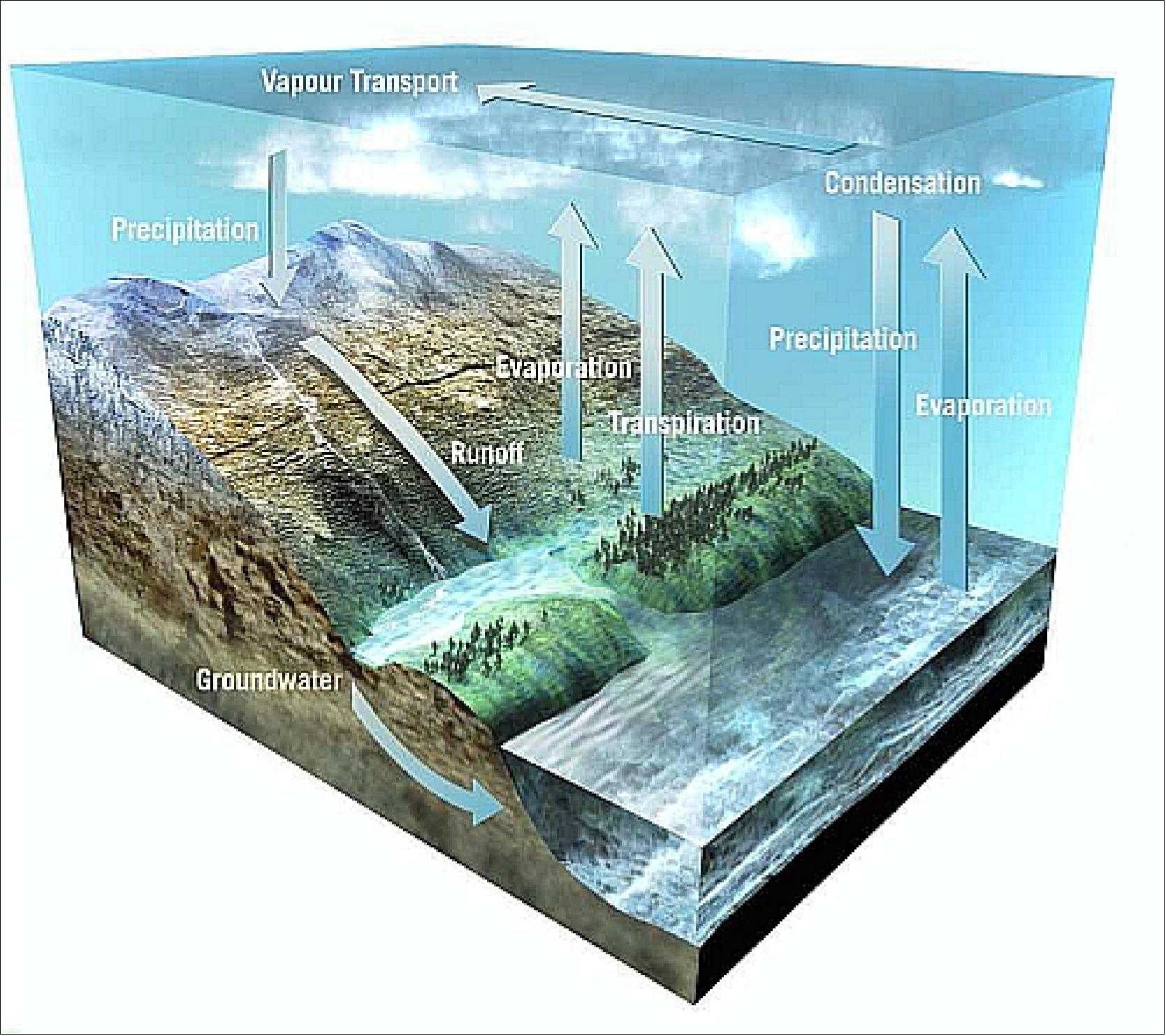
Known as ESA’s ‘Water Mission’, SMOS will improve our understanding of Earth’s water cycle, providing much-needed data for modelling the weather and climate, and increasing the skill in numerical weather and climate prediction. One of the highest priorities in Earth science and environmental policy issues today is to understand the potential consequences of modification of Earth’s water cycle due to climate change. The influence of increases in atmospheric greenhouse gases and aerosols on atmospheric water vapour concentrations, clouds, precipitation patterns and water availability must be understood in order to predict the consequences for water availability for consumption and agriculture. 6)
The main science objective of the SMOS mission is to demonstrate observations of SSS (Sea Surface Salinity) over oceans and SM (Soil Moisture) over land to advance climatologic, meteorologic, hydrologic, and oceanographic applications. Soil moisture is a key variable in the hydrologic cycle. Overland, water and energy fluxes at the surface/atmosphere interface are strongly dependent upon soil moisture. SM is an important variable for numerical weather and climate models as well as in surface hydrology and in vegetation monitoring. Knowledge of the global distribution of salt in the oceans and of its annual and inter-annual variability is crucial for understanding the role of the ocean and the climate system. Ocean circulation is mainly driven by the momentum and heat fluxes through the atmosphere/ocean interface, it is dependent on water density gradients, which in turn can be traced by the observation of SSS and SST (Sea Surface Temperature). 7) 8) 9) 10) 11) 12) 13) 14) 15)
Soil moisture can be retrieved from brightness temperature observations. Due to the large dielectric contrast between dry soil and water, the soil emissivity "epsilon" at a particular microwave frequency depends upon the moisture content. At L-band in particular, the sensitivity to soil moisture is very high, whereas sensitivity to atmospheric disturbances and surface roughness is minimal. 16) 17) 18)
Parameter | Requirement | Comment |
Soil | 0.04 m3 m-3 (i.e. 4% volumetric soil moisture) or better | For bare soils, for which the influence of near-surface soil moisture on surface water fluxes is strong, it has been shown that a random error of 0.04 m3 m-3 allows a good estimation of the evaporation and soil transfer parameters. |
Spatial | < 50 km | For providing soil-moisture maps to global atmospheric models, a 50 km resolution is adequate and will allow hydrological modelling with sufficient detail for the world's largest hydrological basins. |
Revisit time | 2.5 to 3 days | A 3 to 5-day revisit cycle is sufficient to retrieve a dose-zone soil-moisture content and evapotranspiration, provided ancillary rainfall information is available. To track the quick-drying period after the rain has fallen, which is very informative about the soil's hydraulic properties, a one- or two-day revisit interval is optimal. The stipulated 2.5 to 3-day bracket will satisfy the first objective always, and the second one most of the time. |
Observation time |
| The precise time of the day is not critical for data acquisition, but the early morning (about 06:00 h) is preferable when ionospheric effects can be expected to be minimal and conditions are as close as possible to thermal equilibrium. The retrievals will then be more accurate, but dew and morning frost can sometimes affect the measurements. |
For seawater, the dielectric constant is determined by the electrical conductivity and the microwave frequency. The ocean surface emissivity is a function of the dielectric constant and the state of the surface roughness. In principle, it is possible to retrieve SSS from brightness temperature observations. -
Mission requirements call for typical values to resolve specific phenomena:
• Barrier layer effects on the tropical Pacific heat flux: accuracy of 0.2 psu (practical salinity unit), with a spatial resolution of 100 km x 100 km, and a revisit time of 30 days.
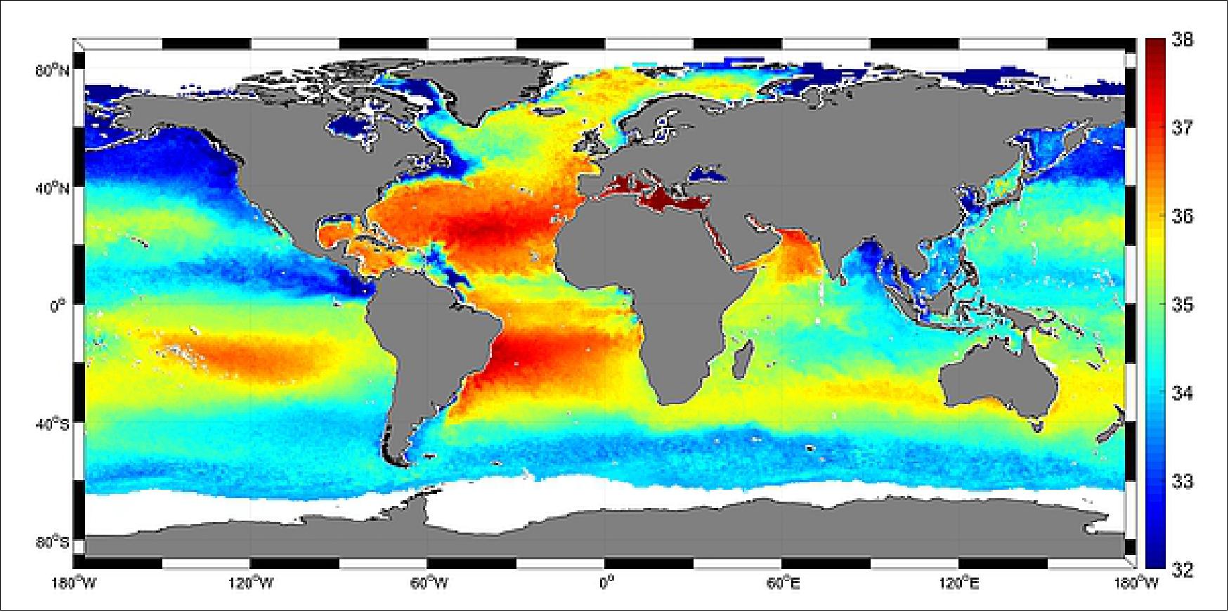
Note: SSS is defined in practical salinity units (1 psu = 0.1%) and ranges from about 32 to 37 psu. In other words, salinity describes the concentration of dissolved salts in water; the psu value expresses the conductivity ratio. The average SSS is 35 psu, which is equivalent to 35 grams of salt in 1 liter of water. The sensitivity of brightness temperature to salinity is about 0.5 K/psu at a water temperature of 20ºC, decreasing to about 0.25 K/psu at 0ºC.
Salinity links the climatic variations of the global water cycle and ocean circulation: 20)
- Salinity is required to determine seawater density, which in turn governs ocean circulation
- Salinity variations are governed by freshwater fluxes due to precipitation, evaporation, runoff and the freezing and melting of ice.
• Halosteristic adjustment of heat storage from the sea level: 0.2 psu, a spatial resolution of 200 km x 200 km, and a repeat cycle of 7 days
• North Atlantic thermohaline circulation: 0.1 psu, a spatial resolution of 100 km x 100 km, and a repeat cycle of 30 days
• Surface freshwater flux balance: 0.1 psu, a spatial resolution of 300 km x 300 km, and a revisit time of 30 days.
Background on SMOS development: Twenty-six years after the first attempt to retrieve soil moisture from space (Skylab L-band radiometer experiment in 1973, referred to as S-194) and following seven years of technology development at ESA (since 1992), the SMOS Earth Explorer Mission was selected for implementation in November 1999 by ESA's Program Board for Earth Observation (PB/EO). Since then, a successful Phase A feasibility study (2000-2001) and a Phase B (2002) for further definition and critical breadboarding have been completed (the Phase B payload design was completed in Oct. 2003). Approval for full implementation was given in Nov. 2003. The SMOS project is now well consolidated, and the payload implementation Phase C/D started in mid-2004. The CDR (Critical Design Review) of the payload took place in Nov. 2005. Delivery of the fully tested payload PFM (Proto-Flight Model) to Alcatel Cannes is scheduled for the end of 2006. 21)
In addition to SMOS, the SAC-D/Aquarius mission is currently under joint development by NASA and CONAE (Argentinian Space Agency). Aquarius will follow up the successful Skylab demonstration mission and employs a combined L-band real-aperture radiometer with an L-band scatterometer. The combined measurements will be focused on the measurement of global sea-surface salinity. A launch of SAC-D/Aquarius is scheduled for 2010. Aquarius will cover the oceans in 8 days with a spatial resolution of 100 km, though its sensitivity to salinity will be better than that of SMOS due to its different design.
Spacecraft
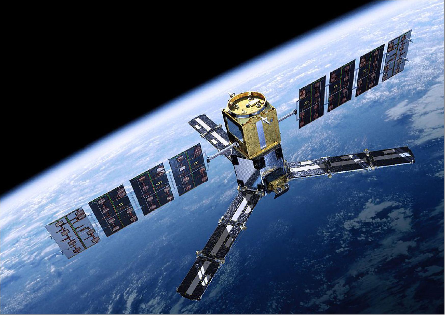
The SMOS satellite uses the generic Proteus bus developed by CNES and Alcatel Alenia Space (formerly Alcatel Space Industries). This standard platform has been designed to accommodate a wide field of missions, orbits, attitudes, instruments, and launch vehicles. Proteus has simple, well-defined interfaces. The platform architecture is generic. Adaptations are limited to minor changes in software modules and the launch vehicle interface.
The S/C bus is a box, nearly 1 m per side, with all the equipment units accommodated on four lateral panels and the lower plate. The platform TCS (Thermal Control Subsystem) relies on passive radiators and active regulation with heaters. Electrical power is generated by two symmetric wing arrays with single-axis step motors. Each wing is composed of four deployable panels (1.5 m x 0.8 m) covered with silicon cells which provide 685 W orbital average after 3-year mission (EOL). The power is distributed through a single non-regulated primary electrical bus (23/36 V) using a Li-ion battery.
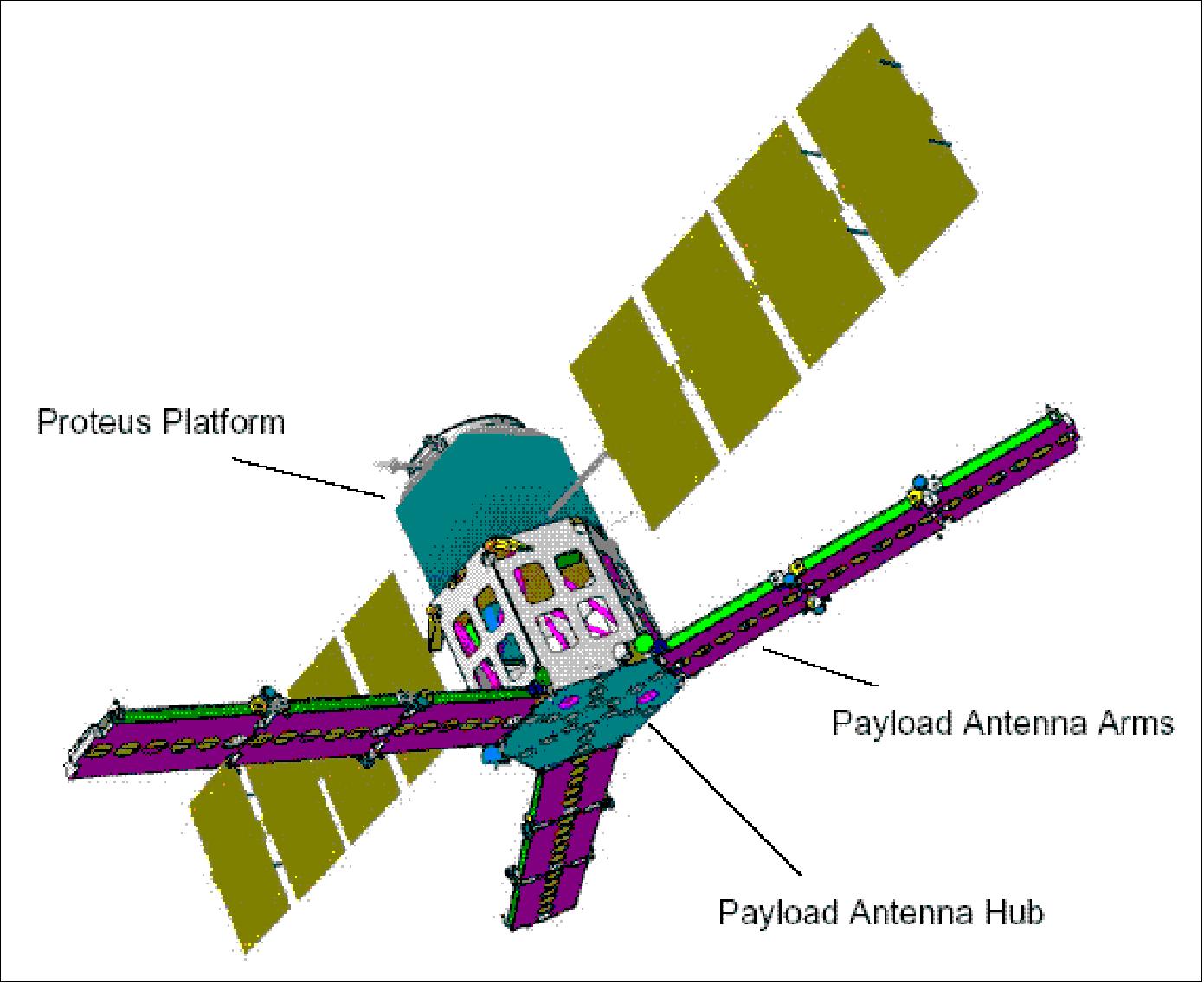
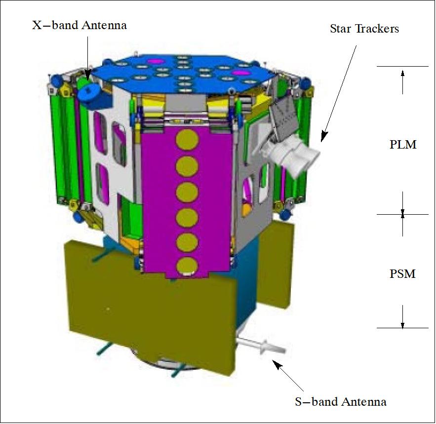
The S/C is three-axis stabilized consisting of a PSM (Proteus Service Module) and a PLM (Payload Module). Typical pointing performance of better than 0.05º (3 σ) is provided by a control system with four reaction wheels and gyro-stellar attitude determination [attitude is provided by two STA (Star Tracker Assembly)]. Coarse sun sensors (8) and two 3-axis magnetometers provide attitude measurement and magnetic torquers generate torque. In addition, two of the four reaction wheels are used to provide gyroscopic stiffness. A GPS receiver provides S/C location data for accurate orbit determinations and onboard time delivery. 22) 23)
Due to the high variety of pointings to be handled with (earth pointing, yaw steering motion, inertial pointing, etc.), the AOCS concept has been based from the beginning on a gyro stellar hybridation with reaction wheel actuators unloaded through magnetotorquer bars, while safe hold mode only relies on kinetic momentum, coarse sun sensors and magnetic sensors and actuators, without the use of the four 1N thrusters in blow down mode limited to orbit control manoeuvres. This design has a proven robust behaviour on all the LEO orbits which have been used in the realized missions.
The onboard command and data handling rely on a fully centralized architecture. The DHU (Data Handling Unit) performs most of the tasks through the central processor running the satellite software. It also supports the management of the communication links with all the satellite units either via discrete point-to-point lines or via a MIL-STD-1553B bus.
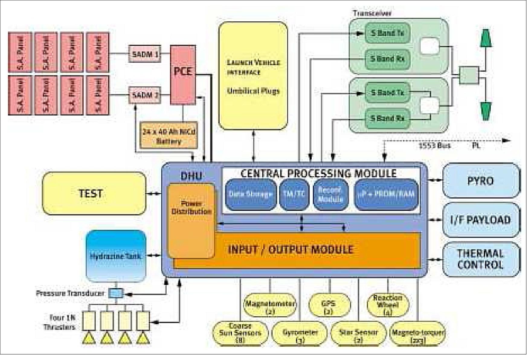
SMOS is designed to operate mostly in an autonomous mode using the FDIR (Failure Detection Isolation and Recovery) concept (this permits to reduce drastically the working hours per day from the ground).
The S/C bus is designed to operate in five distinct satellite modes:
1) normal autonomous operations mode,
2) safe hold mode,
3) star acquisition mode,
4) orbit correction mode with 2 thrusters,
5) orbit correction mode with 4 thrusters.
The SMOS spacecraft has a total mass of 658 kg (bus dry mass of 275 kg, 28 kg of hydrazine, four 1 N thrusters, payload module (PLM) of 355 kg). The design life is three years with a goal of five years.
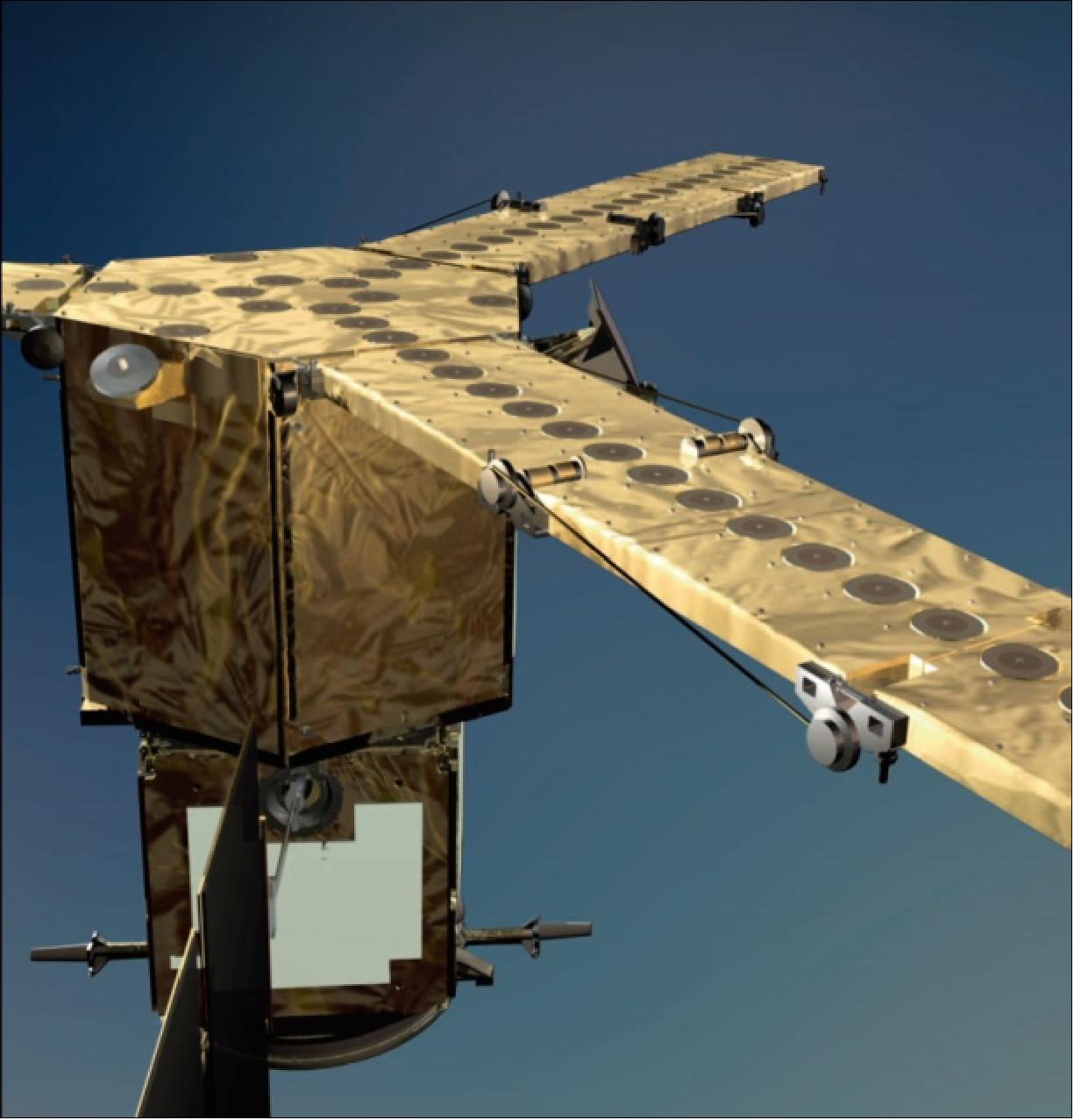
The SMOS spacecraft features an attitude in which the boresight of the antenna is forward tilted by 32.5º with respect to nadir. This configuration enables measurements at line-of-sight angles between 0º - 50º. The satellite employs yaw steering about the local normal.
Spacecraft mass | Launch mass of 670 kg |
Spacecraft power | Up to 1065 W (511 W available for payload); 78 AH Li-ion battery |
Mission duration | Minimum of 3 years |
Spacecraft bus | Proteus platform of CNES |
Payload interface | Dedicated MIL-STD 1553 bus, 160 kbit/s + dedicated TM/TC |
Data storage | 500 Mbit bus + 2 Gbit fpr payload data at EOL (End of Life) |
Spacecraft Operations & Control Center | CNES, Toulouse, France |
Payload Mission and Data Center | ESAC, Villafranca, Spain |
RF communications | S-band for TT&C support, downlink data rate at 722 kbit/s, uplink at 4 kbit/s |
TCS (Thermal Control Subsystem): The TCS is required to maintain all the payload equipment (MIRAS) within the specified temperature range with minimum heater power consumption. The most challenging requirements in operation are relevant to the stringent temperature control of the LICEF (Lightweight Cost-Effective Front-end) receivers. The TCS is based mainly on a passive design, supported by heater systems. All six LICEF receivers in each segment and the eighteen LICEF receivers on the Hub are installed on an aluminum doubler to minimize the gradients among them. 24)
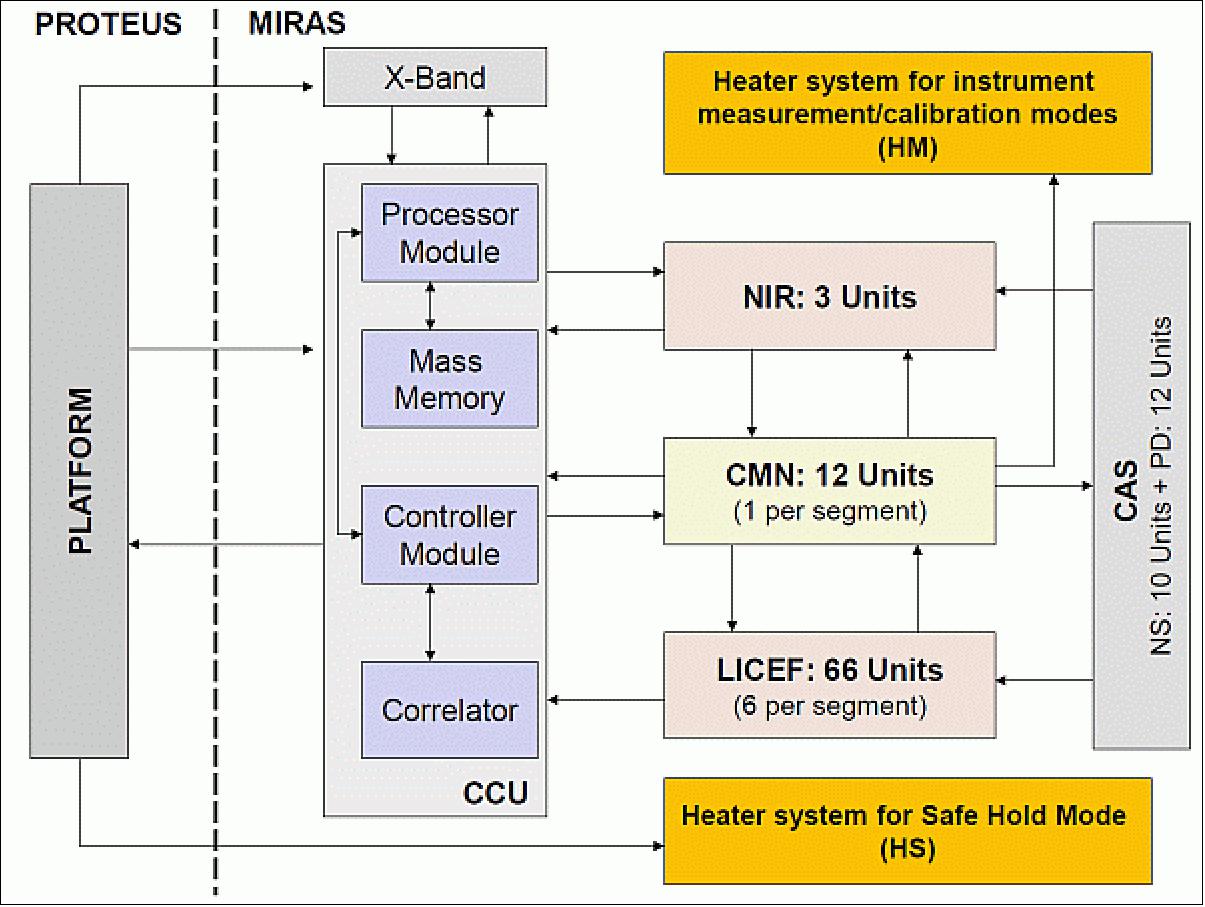
Legend to Figure 5: The TCS has two separate parts:
(1) HM used for Measurement and Calibration Modes and controlled through CCU-CMN (Correlator and Control Unit-Control and Monitoring Node) chain,
(2) HS used for SHM (Safe Hold Mode) and controlled through Proteus platform.
• Passive Thermal Control Design: The passive thermal control hardware incorporates: FSSM (Flexible Second Surface Mirror coatings) for thermal radiators, MLIs (Multi-Layer Insulation Blankets), Germanium-coated black Kapton foil, black paint, aluminized tapes/low emissivity surface treatments, thermal doublers, interface fillers and thermal washers.
• Active Thermal Control Design: The two heater systems in the payload are named HM and HS (Figure 5).
- Electrical resistance heaters (HM in Figure 5) are installed on thermal doublers, on CMN Units and on segments structure and they are powered through CMN commands. This heater system is used to control the electronic equipment temperature in the instrument measurement/calibration modes and in PLM Off modes.
- The HS heaters (Figure 5) are installed on thermal doublers, on CMNs, on CCU, on X-band transmitter, on pyro unit, and on Lower Platform Optical Splitter. The HS heaters are powered from Proteus and controlled by thermostats. This heater system is used to keep equipment temperatures above the minimum non-operational limits (–20 ºC for most of the units) during satellite SHM and PLM Off modes. The system is fully redundant.
The TCS, as well as the rest of the payload design, has a distributed architecture. The central computer of the payload controls in closed loop remotely distributed units (12 in total) named CMN (Control and Monitoring Node) units. Each CMN unit acquires the telemetry of the temperature sensors (6 per heater line) for the heater control lines distributed in the Arms and in the Hub. The TCS is enabled during all payload operational modes including measurement and calibration.
Launch
The SMOS spacecraft was launched on November 2, 2009, on a Rockot launch vehicle (the 3rd stage of Rockot is Breeze-KM) of ELS (Eurockot Launch Services) from the Plesetsk Cosmodrome, Russia. The first burn of Breeze-KM is to acquire an elliptical transfer orbit. The second burn serves to circularize the orbit to its nominal parameters. A secondary payload on this flight is the PROBA-2 spacecraft of ESA. 25) 26) 27)
Some 70 minutes after launch, SMOS successfully separated from Rockot’s Breeze-KM upper stage. Shortly thereafter, the satellite’s initial telemetry was acquired by the Hartebeesthoek ground station, near Johannesburg, South Africa. The upper stage then performed additional maneuvers to arrive at a slightly lower orbit and PROBA-2 was released too, some 3 hours into the flight.
Note: The SMOS satellite has been in storage at Thales Alenia Space's facilities in Cannes, France since May 2008 awaiting a third stage of the Rockot launcher to be assigned to the mission and a slot given for launch from the Russian Plesetsk Cosmodrome. SMOS is the second of ESA's Earth Explorer missions to launch after the GOCE (Gravity field and steady-state Ocean Circulation Explorer), which was launched on March 17, 2009.
Orbit: Sun-synchronous polar orbit, mean altitude = 758 km, inclination = 98.45º, local equator crossing time at 6:00 AM on ascending node maintained within ±15 minutes, period of 100 minutes. The repeat cycle is 149 days. 28)
RF communications: An onboard solid-state recorder has a capacity of 3 Gbit for payload and TT&C data. Standard TT&C S-band communications are used (the downlink data rate is 722.116 kbit/s with QPSK modulation; the uplink has a data rate of 4 kbit/s). The CCSDS protocol is used for TT&C support. - The TT&C station is located in Kiruna (Sweden), operated by CNES (mission operations at CNES). Science data acquisition is in X-band at a data rate of 18.4 Mbit/s, and the ground station is located at Villafranca, Spain.
Mission Status
• January 17, 2024: ESA's SMOS mission, originally designed to study soil moisture and ocean salinity, is now playing a significant role in space weather applications. The mission’s MIRAS instrument, a passive microwave 2D interferometric radiometer, captures L-band signals that contain valuable data on solar flux, allowing researchers to monitor solar activity and its effects on Earth. A newly developed algorithm has been used to extract solar flux measurements at 1.4 GHz from SMOS data, enabling better modeling of space weather events. This information is especially useful for air navigation, space weather modeling, and ionospheric electron content mapping, with validated datasets that show high sensitivity to solar radio bursts. 173)
- During the recent SMOS for Space Weather workshop, researchers discussed several applications of SMOS data in space weather. The solar flux dataset, derived from SMOS observations, was shown to be useful for evaluating the impact of solar flares on GNSS signals, as well as detecting Solar Radio Bursts that interfere with satellite navigation. Additionally, SMOS data has been instrumental in generating Vertical Total Electron Content (VTEC) maps, which are crucial for understanding ionospheric conditions. These applications demonstrate the expanding use of SMOS mission data beyond its original Earth observation goals, highlighting its growing importance in space weather research.
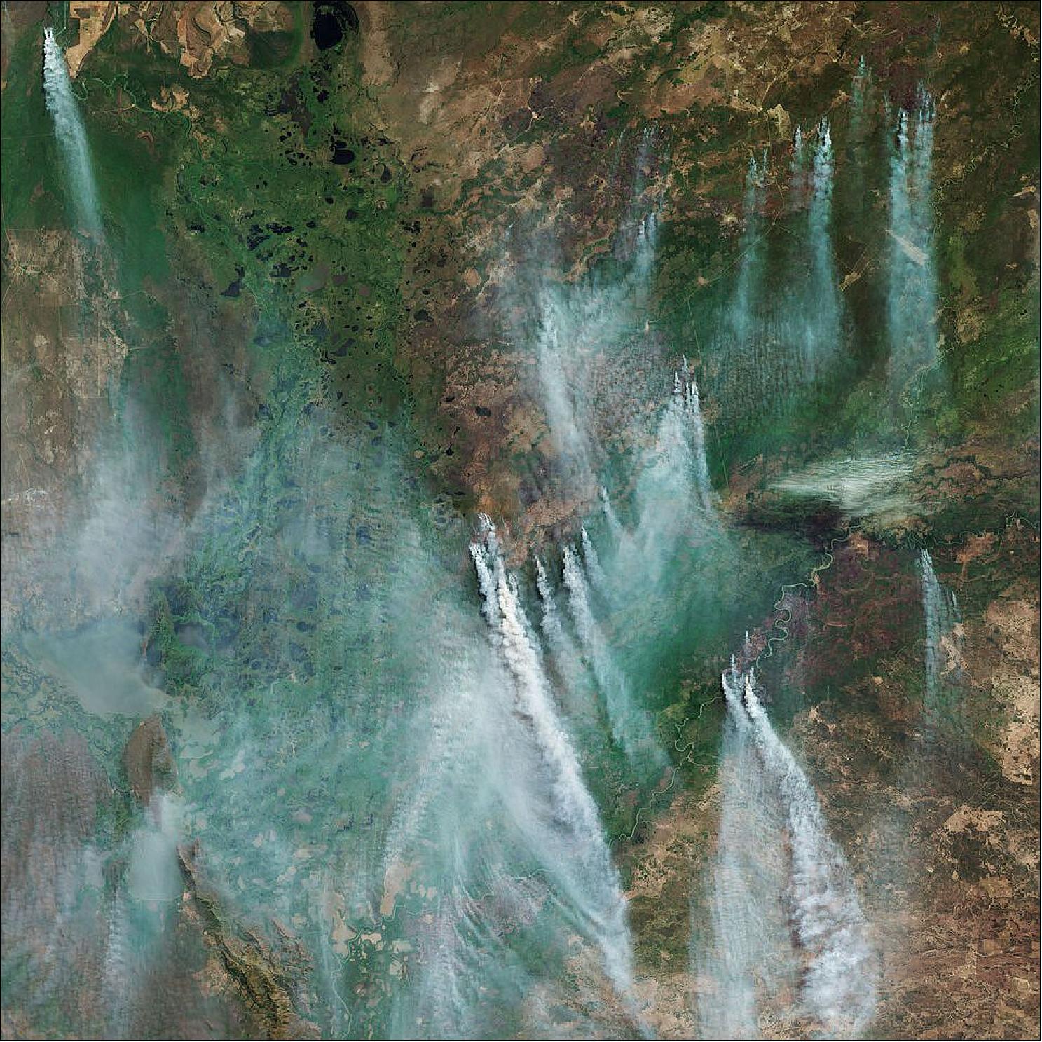
• June 10, 2021: Recent studies using ESA satellite data indicate that forest degradation has become the largest driver of carbon loss in the Brazilian Amazon, surpassing even deforestation. The distinction between the two is crucial: deforestation involves complete clearance of forests, while degradation refers to the decline in forest health, affecting their capacity to absorb and store carbon. A study published in Nature Climate Change reported a cumulative gross carbon loss of 4.45 Pg C in the Amazon from 2010 to 2019, with severe climate events, like the El Niño of 2015, further shifting intact forests from being carbon sinks to significant sources of carbon dioxide. 29) 30)
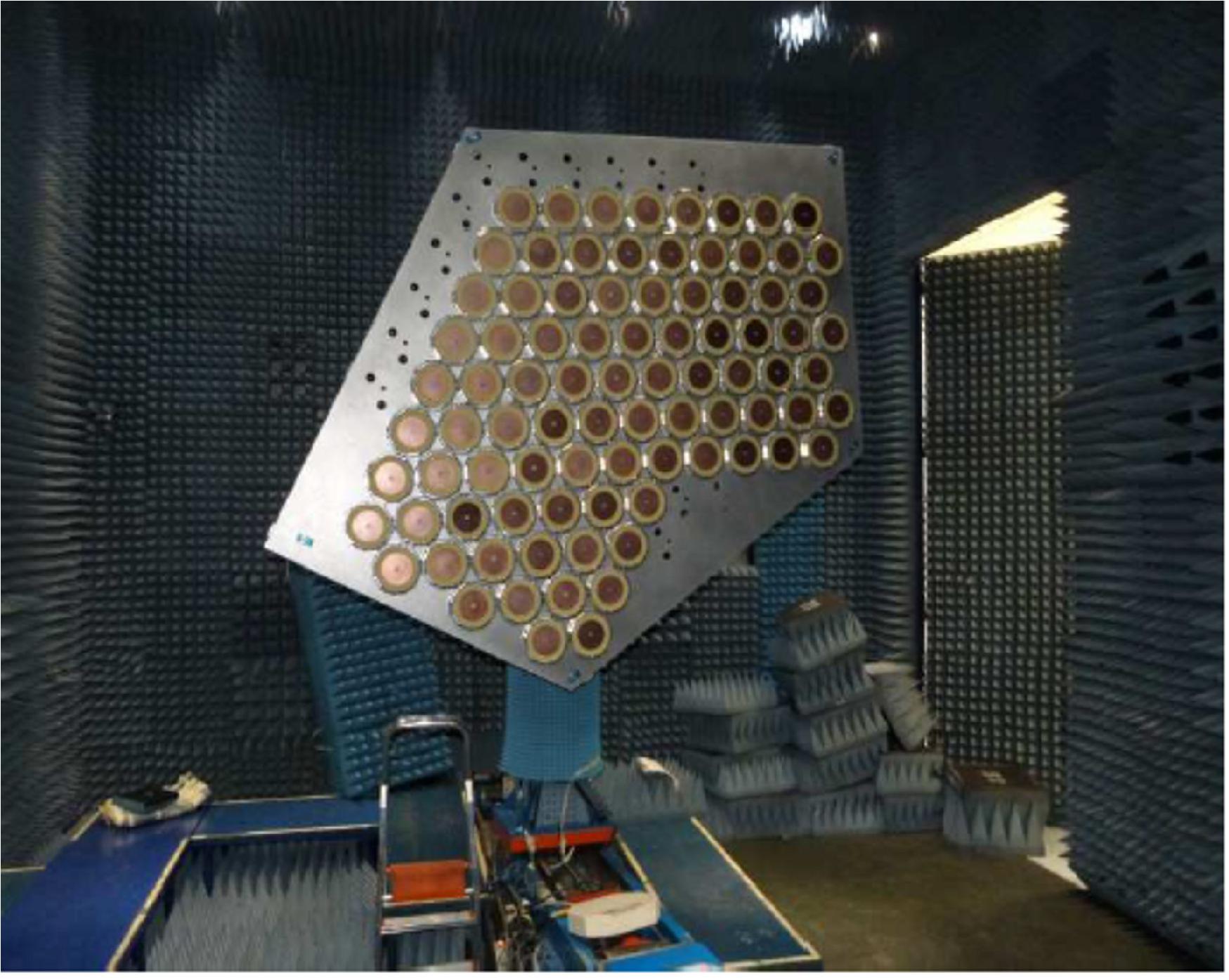
• May 5, 2021: The MIRAS (Microwave Imaging Radiometer using Aperture Synthesis) instrument aboard the SMOS satellite is a passive microwave 2-D interferometric radiometer operating at L-Band (1.4 GHz). It measures faint microwave emissions from Earth's surface to map various geophysical variables, including soil moisture, sea surface salinity, sea ice thickness, wind speed over oceans, and soil freeze/thaw states. MIRAS is unique in that it captures two-dimensional images without the need for mechanical scanning, unlike traditional radiometers. However, different error sources can introduce bias and spatial ripples in the brightness temperature images, which have been studied since before the satellite's launch. 31)
- Recent investigations, aided by SMOS's comprehensive data record, have deepened the understanding of the spatial ripple's origins. A collaborative project involving TDE and Airbus in Spain has demonstrated that an interferometer with a lower spatial ripple can be constructed, enhancing future radiometer missions that utilize aperture synthesis. The experimental results indicate that a two-dimensional radiometer designed with a hexagonal geometry can achieve a noise floor one order of magnitude lower by adjusting the spacing between elements and incorporating ‘dummy’ elements around each active antenna. While adding three rows of dummy elements improved symmetry, adding a fourth row did not yield further enhancements.
• March 24, 2021: For over a decade, ESA’s SMOS satellite has been instrumental in mapping soil moisture and ocean salinity, enhancing our understanding of the water cycle. Beyond its primary functions, SMOS has consistently exceeded expectations, yielding unexpected results that have practical applications in daily life. Recent findings indicate that what was previously considered noise in the satellite's data can actually be utilised to monitor solar activity and space weather, which pose risks to communication and navigation systems. 32)
- The SMOS satellite employs a unique interferometric radiometer that captures signals at a frequency of 1.4 GHz, allowing it to detect emissions from both Earth's surface and the Sun. While the latter usually introduces noise into the brightness temperature images, researchers have discovered that these solar signals can provide valuable insights into solar activity, including solar flares and coronal mass ejections. This capability positions SMOS as a promising tool for monitoring space weather and its potential impacts on Global Navigation Satellite Systems, communications, and power infrastructure. Continued research aims to develop a dedicated retrieval algorithm for these solar signals, further expanding the mission's utility beyond its initial objectives.
• June 23, 2020: Launched over a decade ago, ESA’s Earth Explorer satellite SMOS has not only surpassed its intended lifespan, but has also exceeded its initial scientific objectives. Designed to showcase innovative technology in space and enhance our understanding of Earth’s systems, SMOS has proven invaluable in a range of practical applications. With the increasing prevalence of drought conditions, entrepreneurs are leveraging soil moisture data from SMOS, along with information from other satellites, to create commercial data products for the insurance industry. This initiative is helping to provide essential insights and resources for farmers, enabling them to better manage risks associated with changing climate conditions 34)
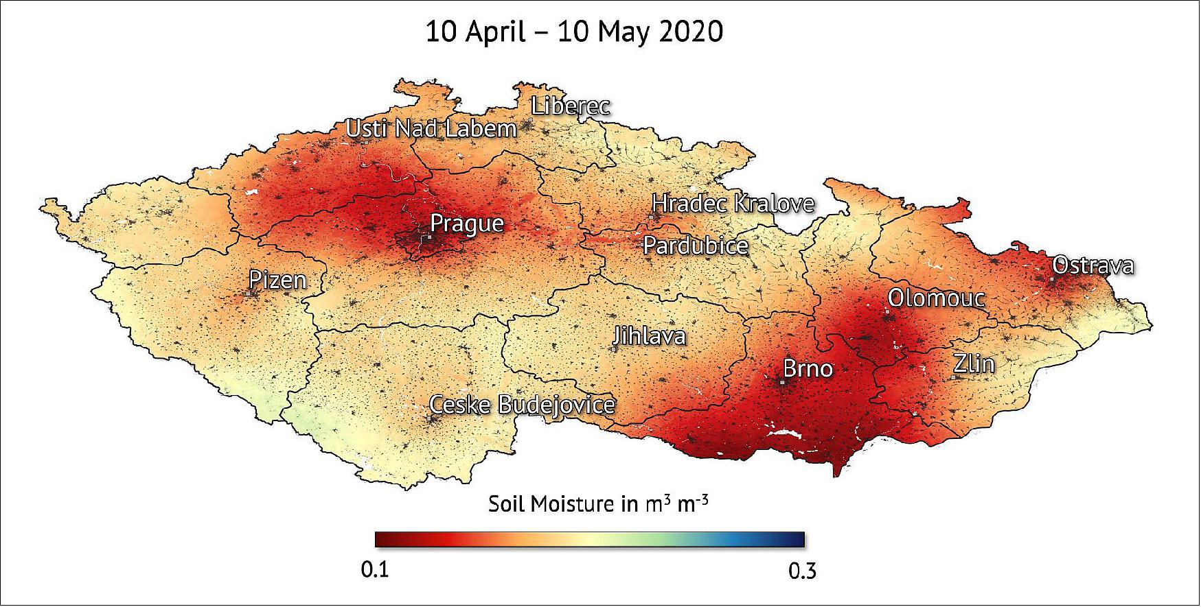
• May 18, 2020: The Czech Republic is currently facing what experts are labeling as the worst drought in 500 years, prompting scientists to utilize ESA satellite data for monitoring purposes. Recent maps produced by VanderSat indicate significantly drier-than-average soil moisture conditions from April to May 2020, with certain areas, particularly in the Olomouc and Ústí regions, exhibiting a 30% decrease compared to the previous six-year average. Such a drastic decline in soil moisture during spring could have catastrophic implications for agriculture and the environment if the drought continues into the summer months. 35)
- Droughts pose substantial natural hazards with far-reaching economic, social, and environmental impacts, and their frequency and severity are increasing due to climate change. The ongoing monitoring of drought conditions is critical, especially in a year projected to be one of the hottest on record. VanderSat utilizes data from ESA’s SMOS satellite along with various other space missions to measure global soil moisture, which aids farmers in protecting their crops against drought impacts. The SMOS satellite, operational for over a decade, continues to provide high-quality data, allowing timely observations that support agricultural practices and insurance measures.
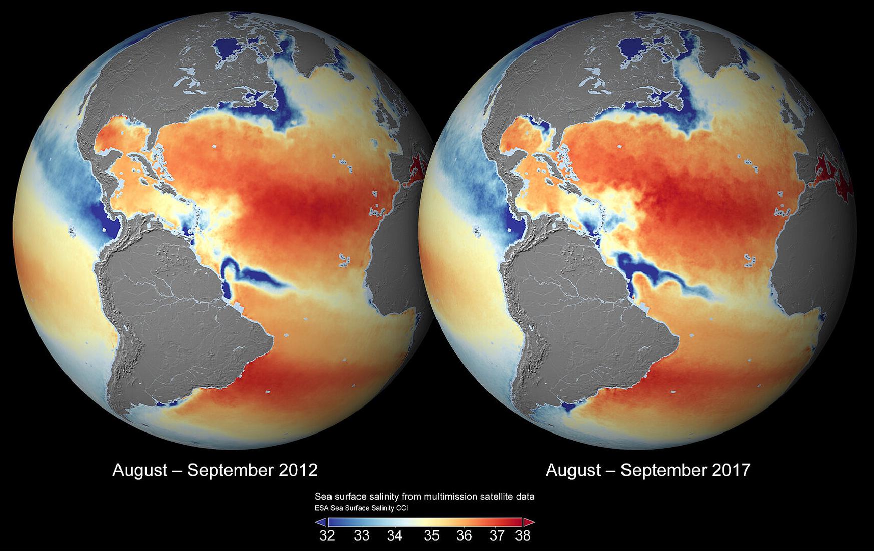
• November 30, 2019: Understanding changes in sea-surface salinity is crucial for comprehending climate change, as variations in salinity influence global climate patterns. Thanks to ESA’s Climate Change Initiative (CCI), scientists have developed the most comprehensive global dataset of sea-surface salinity from space, utilizing data from three satellite missions: SMOS, Aquarius, and Soil Moisture Active Passive. This ongoing project aims to enhance the quality and length of salinity datasets, improving insights into oceanic roles in climate dynamics. The dataset, which spans nine years with weekly and monthly maps at a resolution of 50 km, has achieved a 30% increase in mapping precision through the integration of multiple satellite observations. 36)
• November 28, 2019: This week, the UN World Meteorological Organization announced that greenhouse gas concentrations in the atmosphere have reached new highs, exacerbating global warming and impacting ocean chemistry. As atmospheric carbon dioxide levels rise, the oceans absorb about a third of the carbon emissions from human activities, leading to a decrease in seawater alkalinity, a phenomenon known as ocean acidification. This change disrupts biogeochemical cycles and adversely affects marine life, making it crucial to monitor the current shifts in ocean pH, given that oceans cover over 70% of the Earth's surface and influence overall planetary health. 37)
- While recent advances in monitoring ocean acidification include the use of pH instruments on ships and floats, satellites have not been fully utilized for this purpose. A recent paper published in Remote Sensing of Environment discusses innovative approaches to combining various datasets to estimate ocean acidification, leveraging satellite data from ESA’s SMOS mission and NASA’s Aquarius mission, which provide crucial salinity information. This research, supported by ESA's Earth Observation Science for Society program, aims to continuously monitor ocean carbonate chemistry, identify vulnerable areas, and assess the implications for marine ecosystems and fisheries critical to human food security and economic health. The initiative continues under the ESA's Ocean SODA project as part of the Ocean Science Cluster.
- Traditionally, accurate temperature data within the ice sheet has been sparse, primarily gathered from borehole measurements. Researchers from IFAC-CNR and the Institute of Environmental Geosciences utilized SMOS’s L-band passive microwave observations combined with models to infer temperature profiles at various depths. Their findings indicate that the SMOS satellite provides better estimates of temperature changes with depth, particularly near the bedrock, thus opening new avenues for understanding ice-sheet dynamics that were not possible before. This advancement highlights the satellite's evolving role in climate research and its potential for improving our comprehension of ice behaviour in a changing climate.
• October 31, 2019: SMOS has been in orbit for a decade, exceeding its planned operational lifespan and original scientific goals. Designed to provide crucial data on soil moisture and ocean salinity—key components of Earth's water cycle—it has significantly enhanced our understanding of the exchanges between the Earth's surface and the atmosphere. Beyond advancing scientific knowledge, SMOS is also improving weather forecasts and contributing to climate research, while its data is being utilized in an increasing number of practical applications. 40)
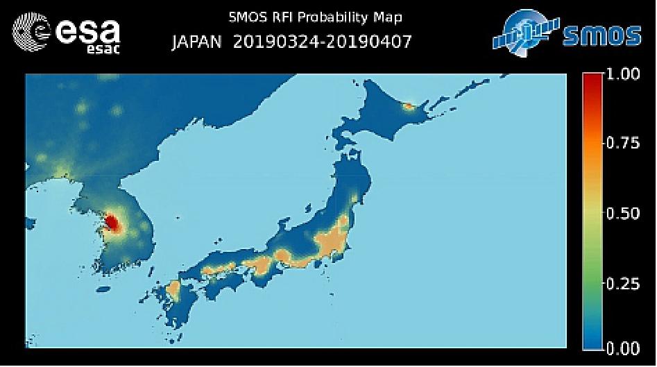
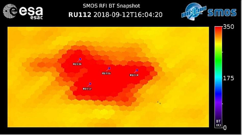
• August 2019: The SMOS (Soil Moisture and Ocean Salinity) satellite, launched by ESA on November 2, 2009, has been operational for nearly a decade, providing crucial data for understanding Earth's water cycle. However, its observations have been significantly impacted by Radio Frequency Interference (RFI), particularly in the passive band of 1400-1427 MHz, where emissions are strictly prohibited by ITU Radio Regulations. The SMOS radiometer has detected various sources of RFI since its initial observations, which are categorized by intensity and emission pattern. Very strong emitters can overwhelm the satellite's instrument, leading to substantial data pollution, especially over ocean areas. Moderate power emitters, while less intense, complicate geolocation efforts due to difficulties in pinpointing their sources. Additionally, omnidirectional and directional antennas associated with broadcasting applications have been identified as significant interference sources, with specific cases in South Korea (Figure 15) where a mix of powerful and weak emitters created extensive interference, and in Moscow (Figure 16), where multiple strong emitters blinded the satellite's data collection across the urban area. 41)
- To address these issues, the SMOS RFI team collaborates with national regulatory authorities to monitor and report instances of harmful interference. Actions taken by spectrum management authorities have led to notable improvements, particularly in regions like Europe, North America, and China, where harmful emitters have been identified and deactivated. The experience gathered from SMOS underscores the critical need to protect the 1400-1427 MHz band from unauthorized emissions. Most interference stems from excessive emissions from radar and broadcasting transmitters in adjacent bands, as well as from unauthorized in-band equipment. It is essential for all parties involved to adhere to regulations prohibiting emissions in this band to preserve the integrity of scientific observations, which are vital for various applications, including climate monitoring and natural disaster response. The proactive efforts of the SMOS RFI team demonstrate the importance of effective management strategies in ensuring high-quality data collection from space.
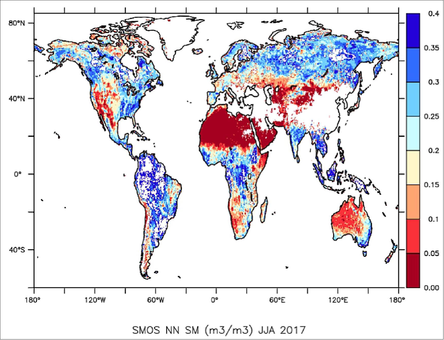
• June 12, 2019: ESA’s SMOS (Soil Moisture and Ocean Salinity) mission has been successfully integrated into the ECMWF (European Centre for Medium-Range Weather Forecasts) forecasting system since its launch in 2009. This integration enhances the accuracy of soil moisture data, which is crucial for effective weather forecasting. Patricia de Rosnay from ECMWF notes that incorporating SMOS measurements improves the understanding of water distribution in the soil and the interactions between land and atmosphere. The system utilizes advanced machine learning techniques, specifically neural networks developed by CESBIO and LERMA, to rapidly process satellite data for operational forecasts. 45)
- Currently, SMOS provides essential data for general weather predictions, as well as for tracking hurricanes and monitoring thin sea ice. This operational use marks a significant milestone, as SMOS is the only Earth explorer satellite contributing to global medium-range weather forecasts. Looking ahead, the potential for integrating additional data from SMOS over oceans and polar regions into Earth-system models could further enhance forecasting capabilities. Matthias Drusch, a mission scientist for SMOS, emphasizes that this integration reflects the ongoing benefits of new satellite observations for operational applications.
• May 14, 2019: Currently, SMOS provides essential data for general weather predictions, as well as for tracking hurricanes and monitoring thin sea ice. This operational use marks a significant milestone, as SMOS is the only Earth explorer satellite contributing to global medium-range weather forecasts. Looking ahead, the potential for integrating additional data from SMOS over oceans and polar regions into Earth-system models could further enhance forecasting capabilities. Matthias Drusch, a mission scientist for SMOS, emphasizes that this integration reflects the ongoing benefits of new satellite observations for operational applications. 46)
- This initiative supports long-term monitoring of essential climate variables, aiding the UN Framework Convention on Climate Change and the Intergovernmental Panel on Climate Change. The dataset not only addresses trends observed since the 1950s—showing saline areas becoming saltier and freshwater areas fresher—but also fills gaps left by traditional in-situ measurements. The team is collaborating with climate scientists to validate this new dataset against in-situ data and model outputs, particularly focusing on climate investigations in the Bay of Bengal to explore salinity's role in ocean stratification and air-sea interactions, thereby improving understanding of the global water cycle and extreme weather events.
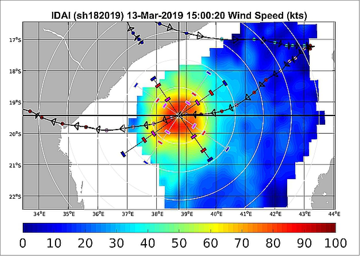
• May 14, 2019: In recent months, Cyclones Fani, Idai, and Kenneth have caused significant devastation, underscoring the urgent need for accurate weather forecasting amid increasing extreme weather events due to climate change. ESA’s SMOS (Soil Moisture and Ocean Salinity) satellite, which has been in orbit for nearly a decade, is expanding its capabilities to enhance storm monitoring and forecasting. Unlike traditional satellites that rely on camera-like instruments unable to penetrate thick cloud cover, SMOS employs a microwave radiometer to capture brightness temperature, enabling it to derive information about ocean salinity and soil moisture, as well as estimate wind speeds during severe storms. 47)
- The unique ability of SMOS to measure ocean-surface wind speeds, even in heavy precipitation, offers a significant advantage, with the potential to improve forecast lead times by 36–72 hours in extratropical regions. To leverage this capability, ESA, OceanDataLab, and Ifremer have launched a pre-operational SMOS wind data service, providing near-real-time wind speed information to organizations like the NOAA National Hurricane Center and the U.S. Naval Research Laboratory. This initiative not only enhances the immediate applications of the SMOS mission but also contributes to the planning of future Copernicus missions focused on critical regions like the Arctic.
• November 2018: ESA, in collaboration with OceanDataLab (ODL) and IFREMER, has initiated a pre-operational SMOS wind data service that provides near real-time ocean surface wind speeds derived from SMOS data, with a latency of 3-6 hours. This service has been tested with expert users, including the NOAA National Hurricane Center, the U.S. Naval Research Laboratory (NRL), and the Joint Typhoon Warning Center (JTWC), to evaluate the utility of SMOS wind data for operational storm forecasting. Initial feedback from these users has been very positive, indicating the service's potential benefits in enhancing storm prediction capabilities. 48)
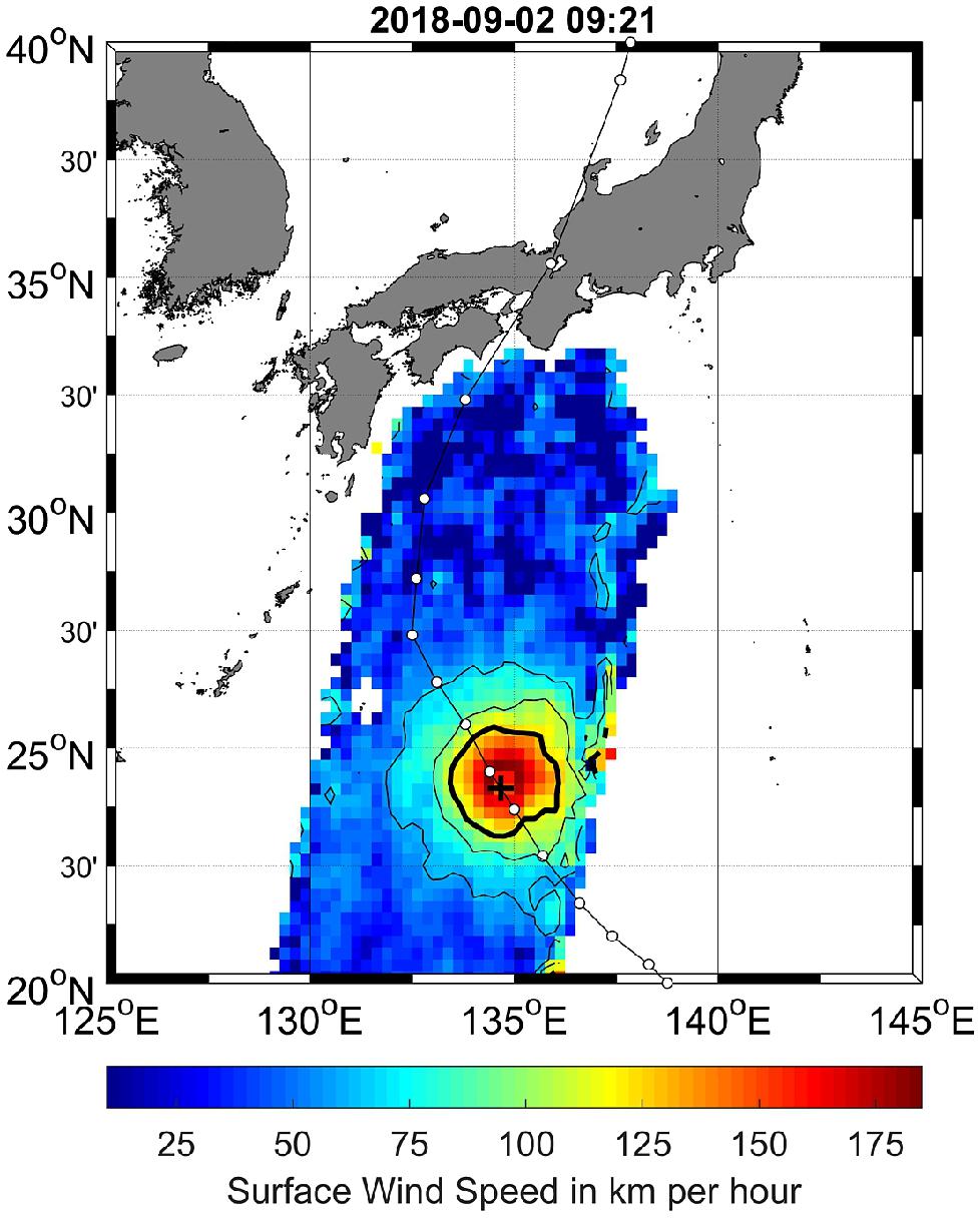
• September 25, 2018: Recent hurricanes and typhoons have highlighted the urgent need for accurate storm path predictions, and ESA’s SMOS (Soil Moisture and Ocean Salinity) mission is poised to enhance forecasting capabilities. While many satellites track storms, SMOS offers a unique perspective by using its microwave sensor to capture 'brightness temperature' images, which reflect radiation emitted from Earth's surface. This technology allows SMOS to detect changes in microwave radiation linked to wind strength, even in storm conditions where traditional optical satellites struggle to see through cloud cover. 49)
- SMOS has recently been tested in operational contexts, providing data on wind conditions during Hurricane Florence and Typhoons Mangkhut and Jebi. Researchers like Buck Sampson from the US Naval Research Laboratory acknowledge that SMOS can contribute valuable information for storm forecasting, which will complement traditional data sources. ESA’s SMOS mission manager, Susanne Mecklenburg, emphasised the potential for SMOS to improve predictions and aid decision-makers in developing effective damage mitigation strategies, thus making a meaningful impact on communities affected by hurricanes globally.
• August 23, 2018: SMOS online Science data are now freely available on the SMOS Online Dissemination Service, without needing to take additional registration steps to access the data. Products can be openly searched and browsed, but an ESA EO-SSO account is required in order to download files. This applies also to users already registered to SMOS data. — Additional information on the available SMOS data and how to access them can be found on the SMOS Data Access page. 50)
• July 2018: ESA's SMOS (Soil Moisture and Ocean Salinity) mission has been in orbit for over 8 years, and its Microwave Imaging Radiometer with Aperture Synthesis (MIRAS) in two dimensions is working well. The data for this whole period has been and is being processed with the operational version of the current Level-1 processor (version v620). Also, a representative part of the same data set has been processed with a working version of a new processor (v720) which is now in preparation so that homogenous records of brightness temperatures have been made available. These rich and long data records have allowed learning important lessons from the in-flight experience, and shall eventually lead to the consolidation of the new Level-1 processor version (v720) with its corresponding auxiliary calibration and configuration files. Once the improvements are confirmed the new processor version shall be recommended for the operational chain. 51)
- The over 8-year flight experience of SMOS is very valuable for the definition of future L-band missions, in particular but not only, in the context of an interferometric radiometer. The lessons learnt tell how SMOS could be improved to attain better sensitivity, spatial resolution, swath (coverage or revisit time), robustness against RFI and stability. The improvements include system parameters such as element spacing or array geometry, subsystem improvements at all levels (antenna, receiver, harness and correlator), as well as calibration approaches and image reconstruction. In summary, the SMOS experience could be used to define a cost-effective SMOS follow-on mission.
• July 2018: ESA's SMOS (Soil Moisture and Ocean Salinity) mission, operational for over eight years, utilises its Microwave Imaging Radiometer with Aperture Synthesis (MIRAS) effectively. Throughout this period, data has been processed using the current Level-1 processor (version v620), with a representative subset also processed by a new version (v720) to ensure consistent brightness temperature records. Insights gained from this extensive data collection will inform the development of the new Level-1 processor, including necessary calibration and configuration files. These lessons will also guide enhancements for future L-band missions, focusing on improved sensitivity, spatial resolution, swath coverage, resistance to radio frequency interference (RFI), and overall stability, which can aid in defining a cost-effective follow-on mission for SMOS. 52)
• April 11, 2018: A new methodology combining debiased non-Bayesian retrieval, DINEOF (Data Interpolating Empirical Orthogonal Functions), and multifractal fusion has produced six years of Sea Surface Salinity (SSS) fields from SMOS data over the North Atlantic Ocean and the Mediterranean Sea. This product was developed by the Barcelona Expert Center and the GHER (GeoHydrodynamics and Environment Research) group at the University of Liège, Belgium, as part of the ESA STSE project "SMOS sea surface salinity data in the Mediterranean Sea (SMOS+ Med)," led by Dr. Aida Alvera-Azcarate from GHER. 53) 54)
• September 2017: Mission operations have been extended through 2019, with a review planned for 2018 to assess further extensions. CNES is evaluating the continuation of operations beyond 2017. Anticipated future data products include severe wind speed measurements over oceans and freeze/thaw information over land. Notably, radio frequency interference has decreased significantly, particularly in Europe, with over 70% of interference sources successfully switched off. 55)
• September 5, 2017: Central Italy is experiencing a severe drought, with satellite data revealing abnormally low soil moisture levels, particularly in southern Tuscany, where conditions have been drier than normal since December 2016. The first half of 2017 recorded less than half of the average rainfall, leading to significant agricultural damage and prompting discussions of potential water rationing in Rome. The Italian Research Institute for Geo-Hydrological Protection (IRPI-CNR) is actively monitoring the situation using a new satellite soil moisture dataset developed by the Vienna University of Technology and VanderSat B.V., which is part of the European Space Agency's Soil Moisture Climate Change Initiative.56)
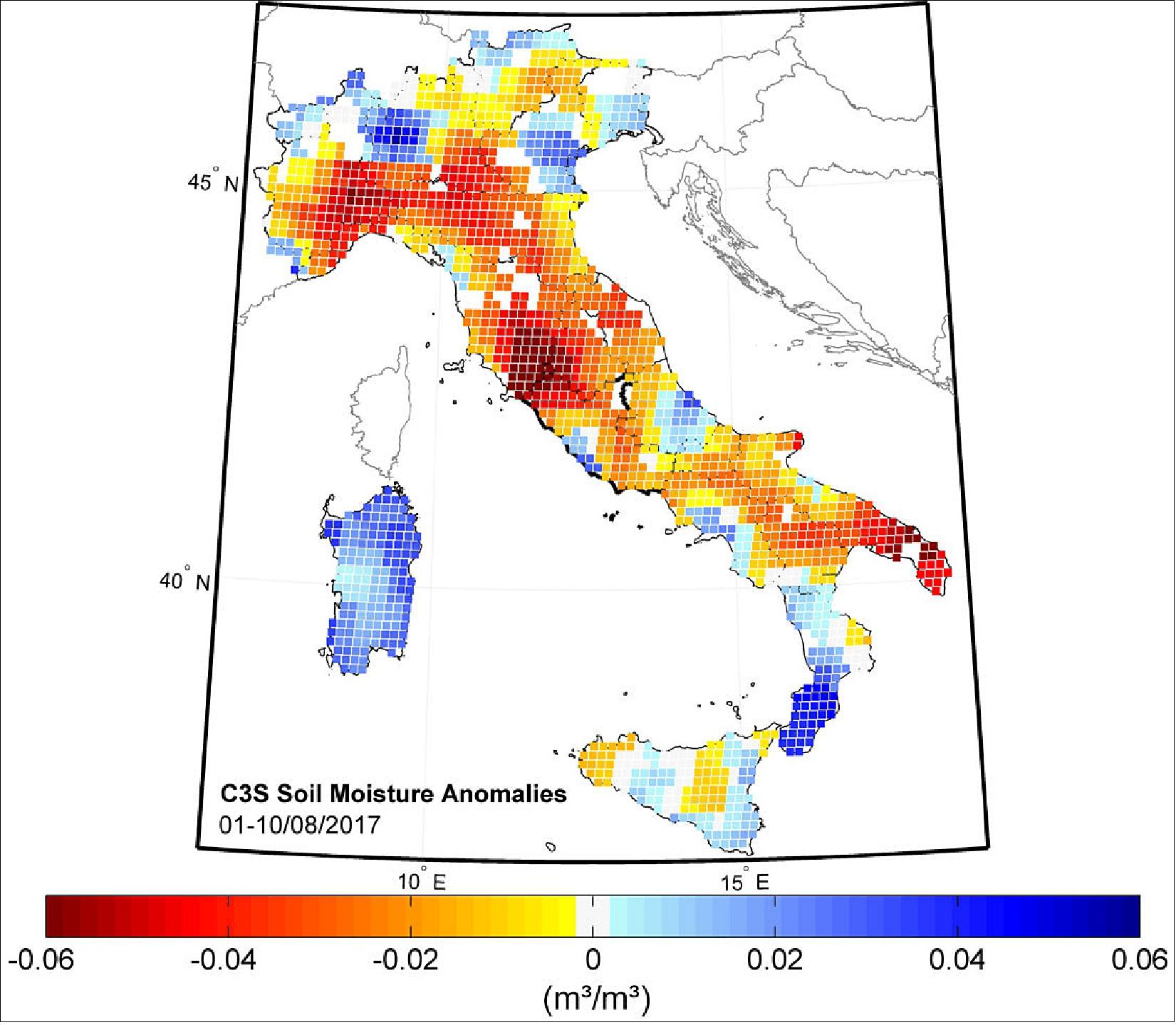
Legend to Figure 24: Soil moisture in Italy during early August 2017 was particularly low in some areas (red). The data were compiled by ESA’s Soil Moisture CCI project and includes information from active and passive microwave sensors (such as those on the ERS, MetOp, SMOS, Aqua and GCOM-W1 satellite missions).
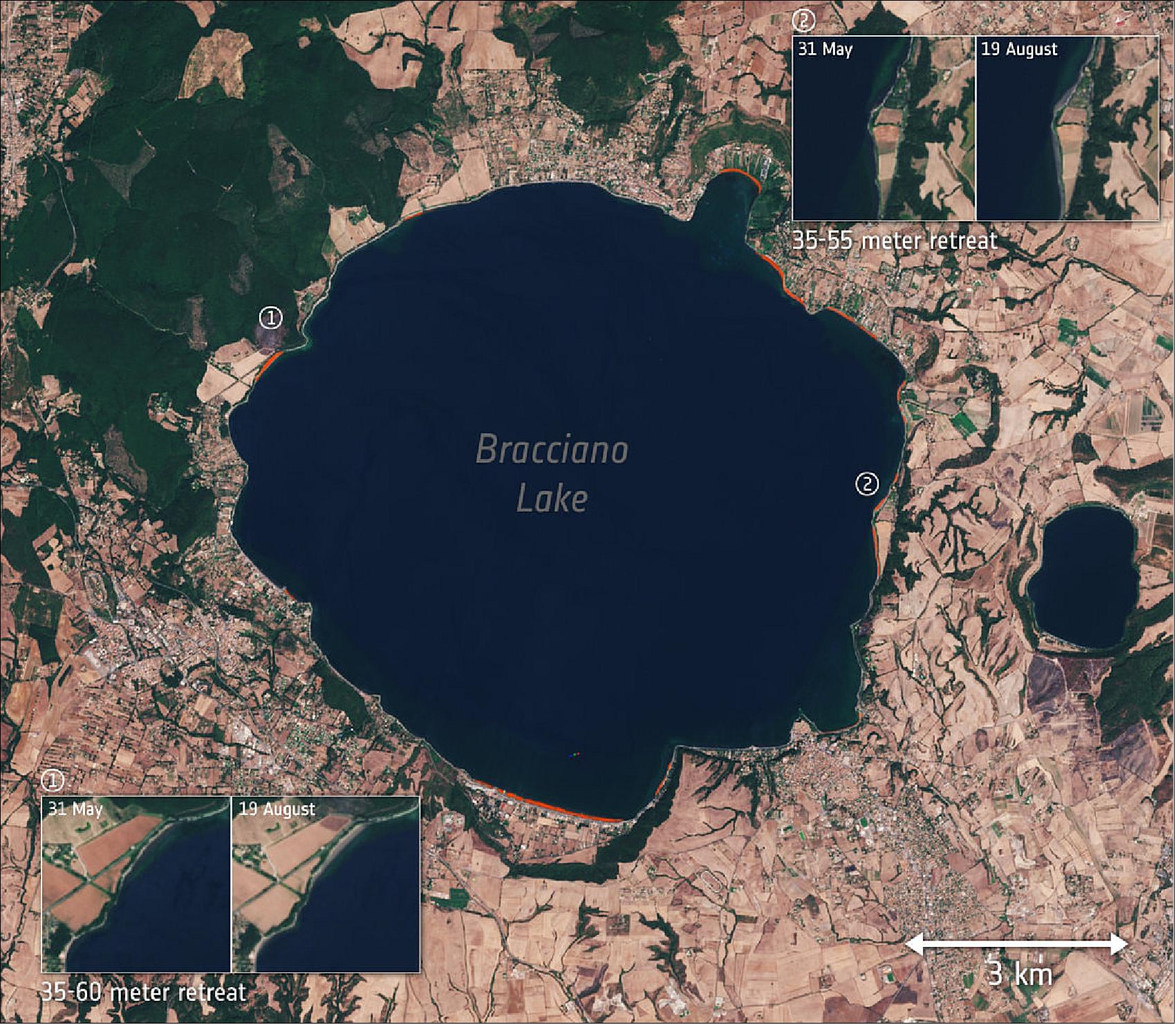
- In addition to soil moisture monitoring, satellites are tracking the effects of the drought on water bodies, including a notable drop in water levels at Lake Bracciano, which is becoming increasingly visible in satellite imagery. While local authorities closely monitor this lake, satellite radar altimeters are also being used to assess water levels in lakes worldwide, enhancing resource management efforts. Scientists continue to leverage space-based tools to monitor drought conditions across Europe and provide support to authorities addressing water scarcity challenges.
• July 2017: ESA's SMOS mission has been operational for over seven years, during which its MIRAS (Microwave Imaging Radiometer with Aperture Synthesis) instrumentation has provided significant insights into its performance and capabilities. This period has allowed researchers to identify effective components, areas requiring improvement, and potential enhancements for future iterations of the instrument. The lessons learned from the mission are categorized into several main topics, including Radio-Frequency Interference (RFI), brightness temperature over the ocean, spatial resolution over land, calibration strategies, and open areas for further exploration. 57)
- One major challenge identified is RFI in the 1400-1420 MHz band, which has been compromised by illegal emissions and faulty equipment. ESA has undertaken significant efforts to mitigate these issues, although many sources remain active. Future missions must integrate RFI mitigation measures at various levels, including array geometry and onboard electronic countermeasures. In terms of brightness temperature, SMOS ocean images are influenced by several factors, such as spatial ripple and land-sea contamination. Enhancements in sensitivity and antenna design could improve data quality. Additionally, while the current spatial resolution over land is 41 km, new geometric arrangements, such as hexagonal arrays, could provide better resolution for hydrological applications. Calibration strategies also present opportunities for improvement, particularly through the removal of Noise Injection Radiometer units, centralizing the calibration process, and reducing temporal fluctuations in detector outputs. Finally, ongoing research aims to better understand the underlying mechanisms of the efficiency factor related to land-sea contamination and to address the noise floor limit affecting spatial ripple in SMOS images.
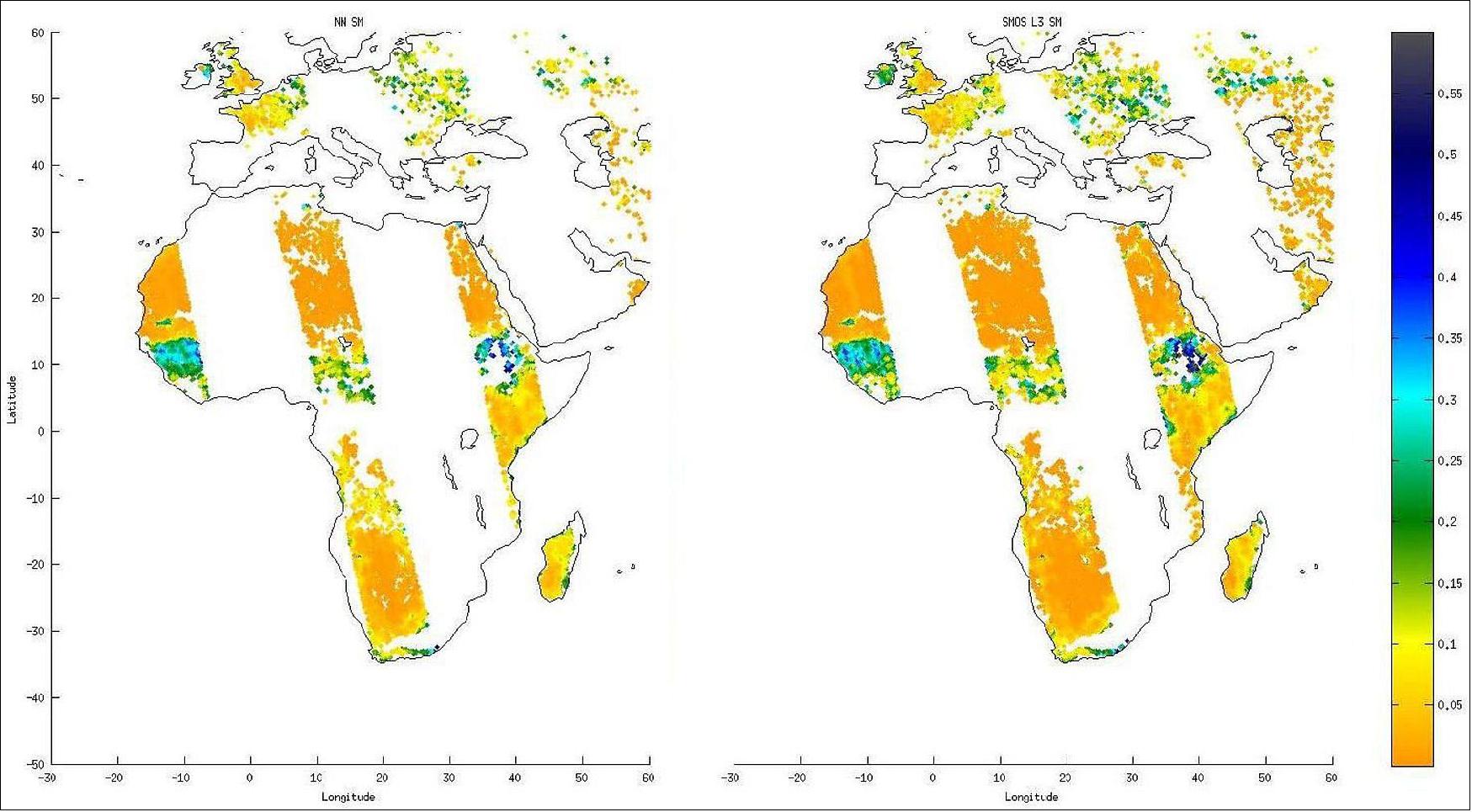
• June 13, 2017: Satellites are playing a crucial role in predicting conditions conducive to desert locust swarming, which threatens agricultural production, livelihoods, and food security. Desert locusts, typically harmless grasshoppers found mainly in the Sahara and surrounding regions, can cause significant crop damage when they swarm. For instance, during the 2003–05 plague in West Africa, over eight million people were affected, with devastating losses to cereals, legumes, and pastures. Swarming occurs following droughts and subsequent rains, leading to rapid vegetation growth, overcrowding, and increased breeding, making locusts particularly dangerous. A single 1 km² swarm can contain about 40 million locusts, consuming as much food in a day as 35,000 people. 58)
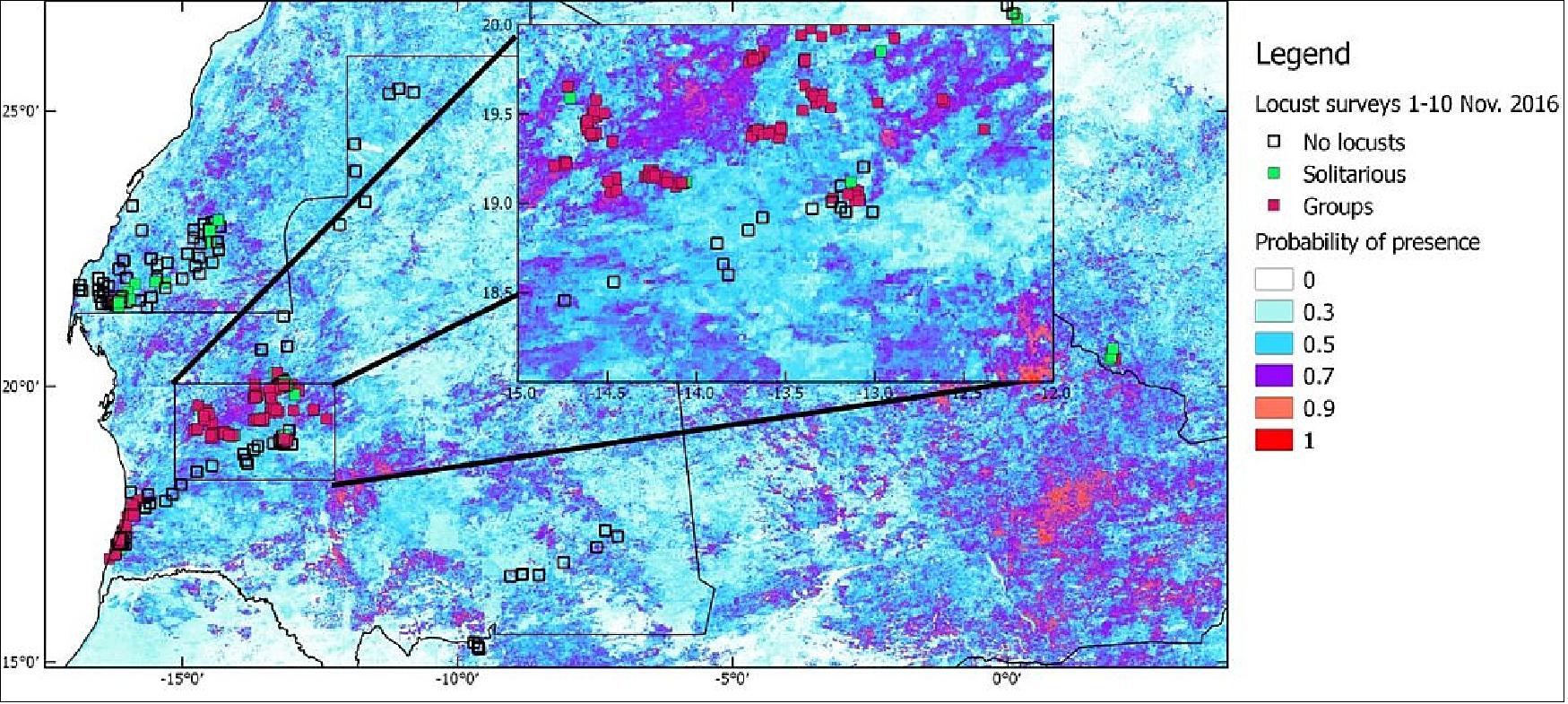
- To improve forecasting of locust plagues, ESA has partnered with international organizations to utilize satellite data, including the SMOS (Soil Moisture and Ocean Salinity) mission. By monitoring soil moisture and green vegetation, the SMOS satellite captures brightness temperature images that provide crucial information at a resolution of 50 km per pixel. By combining this data with medium-resolution information from NASA’s MODIS satellites, the team successfully downscaled soil moisture measurements to a resolution of 1 km per pixel, enabling the prediction of locust-friendly conditions up to 70 days before a November 2016 outbreak in Mauritania. This advance allows authorities to prepare preventive measures in a timely manner, significantly improving the forecasting process compared to previous methods that only provided a one-month warning. Future integrations with the Copernicus Sentinel-3 mission and further enhancements using Sentinel-1 observations aim to provide even more detailed locust forecasts, further aiding efforts to combat potential outbreaks.
• May 11, 2017: ESA’s SMOS mission is designed to map variations in soil moisture and ocean salinity, and it has exceeded expectations by successfully measuring salinity in smaller seas like the Mediterranean. Utilizing a microwave instrument to capture images of brightness temperature, SMOS provides essential data for understanding the Earth’s water cycle and has applications in tracking hurricanes, measuring polar ice, and improving crop yield forecasts. While its measurements enhance our understanding of ocean responses to climate change and phenomena like El Niño, the Mediterranean offers a unique environment for studying shorter-term ocean dynamics, such as the formation of the Alboran Gyre from Atlantic water flow. 59)
- Despite challenges like land-sea contamination and unexpected radio interference from illegal transmitters, efforts by scientists and collaborations with frequency protection authorities have allowed SMOS to effectively map salinity in much of the Mediterranean. Innovations from the Barcelona Expert Center and the University of Liege have led to improvements in data processing techniques, enhancing the accuracy of salinity measurements. Susanne Mecklenburg, the SMOS mission manager, commended these advancements, highlighting how they broaden the mission's applications and showcase SMOS's potential to contribute significantly to scientific understanding and societal benefits.
• December 16, 2016: Although ESA's SMOS satellite was not originally designed for ice detection, it can identify thin sea ice, and when combined with measurements from CryoSat-2, it provides a more detailed understanding of changes in the Arctic. SMOS captures brightness temperature images using a radiometer, which are traditionally utilized to assess soil moisture and ocean salinity but can also be applied to measure thin sea ice. In contrast, CryoSat-2 employs a radar altimeter to accurately determine the freeboard of thicker ice. Researchers from the University of Hamburg and the Alfred Wegener Institute have successfully merged data from both satellites, enhancing the understanding of ice thickness changes. SMOS’s daily images offer valuable but coarser coverage compared to CryoSat-2's high-resolution monthly data. 60)
- This collaboration enables the production of daily maps of Arctic sea ice thickness, significantly improving forecasting for marine traffic operators navigating routes like the Northwest Passage, which are becoming increasingly accessible due to climate change. Additionally, the integration of both missions’ historical data since 2010 contributes to ongoing studies of the Arctic's fragile ice system, with potential benefits for models of ocean currents and air temperatures. Combining these different types of measurements not only advances scientific understanding but also enhances.
- This collaboration enables the production of daily maps of Arctic Sea ice thickness, significantly improving forecasting for marine traffic operators navigating routes like the Northwest Passage, which are becoming increasingly accessible due to climate change. Additionally, the integration of both missions’ historical data since 2010 contributes to ongoing studies of the Arctic's fragile ice system, with potential benefits for models of ocean currents and air temperatures. Combining these different types of measurements not only advances scientific understanding but also enhances.
• October 14, 2016: ESA's SMOS mission is significantly advancing our understanding of Earth while also delivering crucial near-real-time soil moisture data, available within three hours of measurement, which is essential for applications such as weather prediction and flood forecasting. By utilising an artificial neural network to rapidly translate brightness temperature measurements into soil moisture products, SMOS enhances the speed and efficiency of data processing. This swift availability facilitates the integration of SMOS data with information from other satellites, such as NASA's SMAP and Copernicus Sentinel-1, allowing for improved spatial resolution from 25 km x 25 km to 100 m x 100 m. This enhanced data fusion not only supports informed decision-making in agriculture and hydrology but also proves invaluable for monitoring crops, predicting weather patterns, and managing disaster risks, ultimately benefiting over 3,000 users who rely on these critical insights. 61) 62) 63)
• July 2016: The SMOS mission has reprocessed its MIRAS data from over six years using a new fully polarimetric Level-1 processor (v620), enhancing instrument performance and calibration. This update has clarified observations and paved the way for an even more advanced processor version (v700). Key improvements include addressing systematic spatial ripple caused by antenna spacing and patterns and reducing contamination from Sun and Radio Frequency Interference (RFI). The new ALL-LICEF branch in v700 has effectively corrected land-sea contamination, while empirical techniques have improved sea surface salinity retrieval. Orbital variations are now constrained within ±0.4 K, though challenges remain during eclipse seasons. Seasonal variations have been linked to reflected galaxy signals rather than instrument instability. Additionally, a refined in-orbit calibration strategy has optimized external maneuvers to mitigate thermal impacts, enhancing noise calibration consistency. Continuous advancements in image reconstruction techniques are expected to yield further improvements in the upcoming Level-1 processor version (v710). 65)
• Summer 2016: After over six years in orbit, the SMOS mission remains in excellent technical condition, providing high-quality data to both scientific and operational communities. Extended until 2017 by ESA and CNES, the mission faces no technical limitations for further extensions beyond this date. SMOS has achieved its objectives over land, delivering precise soil moisture observations that aid in monitoring floods and droughts and assessing storm risks. Notably, it is expected to serve as a benchmark for generating long-term data records. New products have been introduced, including sea ice thickness for climate research and ship routing, near-real-time soil moisture data for hydrological applications, and severe wind data to enhance storm forecasts. While Radio Frequency Interference (RFI) contamination has been reduced in Europe and the Americas, challenges remain in Asia and the Middle East. 66)
• October 2015: The SMOS mission is enhancing our understanding of rainfall dynamics by providing novel two-dimensional images that capture the imprint of rain on sea surface salinity (SSS) immediately after rain events. These observations complement traditional in situ measurements and satellite rain assessments, which can be difficult due to the irregular nature of rainfall. SMOS SSS effectively serves as a tracer for instantaneous rain rates, exhibiting a linear relationship with rates from individual satellites using RemSS retrieval methods. At moderate wind speeds (3 to 12 meters per second), the rain signature on SMOS SSS shows a change of about -0.2 practical salinity units per millimeter per hour, reflecting a dependency comparable to in situ SSS measurements. 67)

• September 30, 2015: ESA's SMOS mission, alongside NASA's SMAP and Japan's GCOM-W satellites, is enhancing our understanding of surface winds under tropical storm clouds in the Pacific Ocean. This collaboration comes at a critical time, as a strong El Niño is causing higher-than-normal surface ocean temperatures, contributing to an active hurricane season. With eight major hurricanes already recorded, including three category-4 hurricanes near Hawaii, there is an urgent need for accurate marine weather forecasting. SMOS, originally designed for measuring soil moisture and ocean salinity, is now being utilized to monitor wind speeds over the ocean, providing crucial data for predicting storm paths and informing mariners of potential dangers. 69)
- By integrating measurements from these three satellites, scientists are gaining unprecedented insights into how surface wind speed evolves in the presence of tropical storms. This detailed information is essential for improving initial conditions used in hurricane forecasting models, which can enhance the accuracy of storm predictions. Additionally, observations of sea-surface temperatures have revealed cold-water wakes trailing the recent hurricanes, indicating the significant impact of hurricane winds on ocean dynamics. While this synergy among satellite data promises to improve marine and hurricane forecasting, the future of such measurements remains uncertain without guaranteed follow-on missions, underscoring the need for continued investment in satellite technology to monitor ocean-atmosphere interactions.
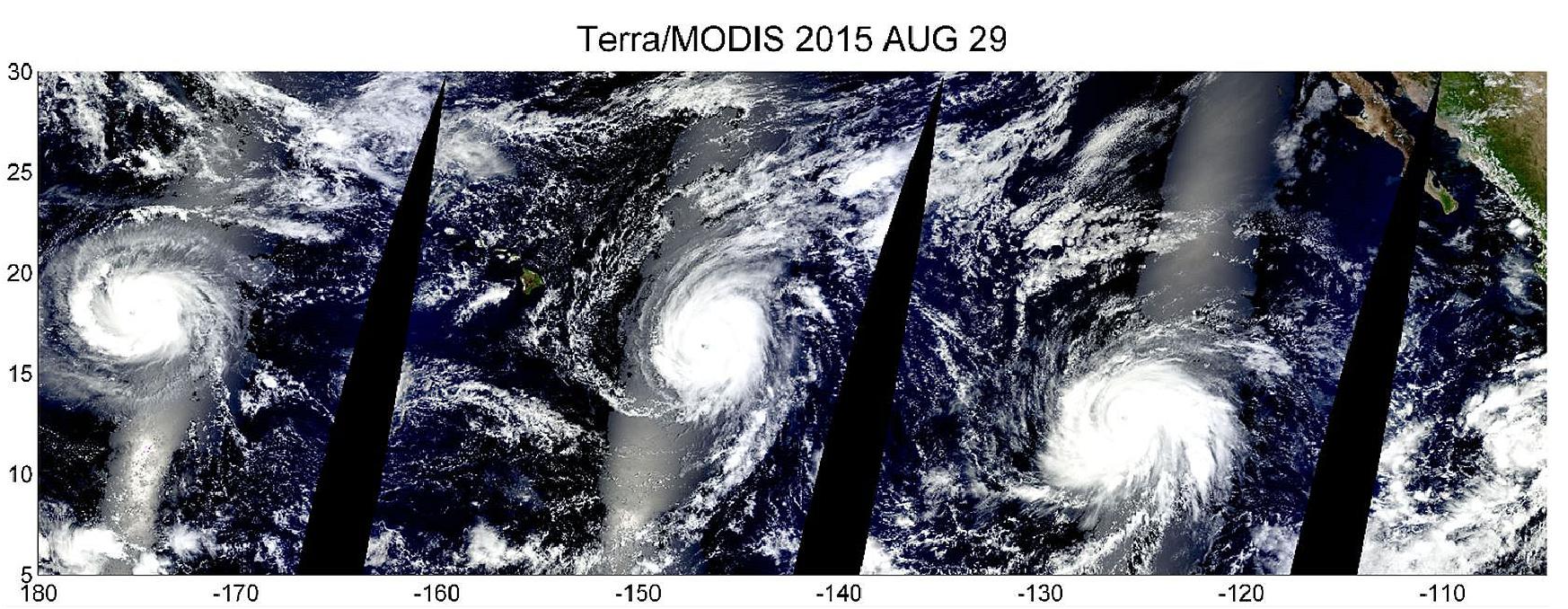
Legend to Figure 34: All three were category-4 hurricanes and spanned the central and eastern Pacific basins. The bright bands in the images are sunglint where solar radiation from the Sun has reflected from Earth back to the satellite sensor. The Copernicus Sentinel-3A satellite, expected to be launched in late 2015, will provide images such as these at 300 m resolution and in 21 bands from its OLCI (Ocean and Land Color Imager) along with thermal infrared images from its SLSTR (Sea and Land Surface Temperature Radiometer).
• August 2015: After more than five years in orbit, the SMOS mission has demonstrated reliable instrument operations, data processing, and dissemination, prompting the extension of its mission through 2017. This extension allows for the ongoing provision of observation datasets, essential for developing pre-operational applications and facilitating their use by operational users. Notably, the mission has added a new objective of providing daily sea ice thickness estimates, showcasing the significant potential of SMOS data for operational applications. The MIRAS instrument, which employs a newly reprocessed fully polarimetric Level-1 processor, has shown improved performance in data quality, including reduced spatial tilt in images and enhanced retrieval of critical geophysical parameters. However, challenges remain, particularly concerning the mitigation of side lobes and radio frequency interference. 70) 71)
- In terms of data biases, the latest processor version has resulted in slightly warmer ocean images, increasing the average deviation from geophysical models. Despite this bias, the accuracy of sea surface salinity retrievals remains unaffected due to corrective measures in the Ocean Target Transformation. Land-sea contamination continues to be an issue, largely linked to calibration errors, although empirical corrections based on brightness temperature records show promise. Additionally, advancements in calibration strategies have improved the long-term stability of the data, mitigating previous drifts and reducing seasonal variations. The SMOS Calibration and Level-1 Processor team is actively exploring new algorithms and models to enhance data accuracy and address ongoing challenges, contributing to the overall mission's success and utility. 72)
• July 2, 2015: ESA's SMOS mission continues to provide essential data on soil moisture and ocean salinity, demonstrating significant societal benefits through its applications in real-world scenarios. The continuity of L-band observations is crucial for operational agencies and numerical weather prediction, as highlighted during the 2nd SMOS Science Conference in May 2015. Agencies such as Mercator Ocean and ECMWF emphasised the potential of SMOS data for enhancing weather forecasting and climate services. For example, the Deputació de Barcelona has successfully integrated SMOS soil moisture data into their summer forest fire prevention campaigns, achieving an 87% detection rate for areas at risk of wildfires, showcasing the mission's practical impact on public safety and resource management. 73)
- In addition to its terrestrial applications, SMOS data have also been utilized to assess sea ice thickness in Arctic waters, critical for navigation in ice-prone regions. Researchers at the University of Hamburg have incorporated these observations into computer models, significantly improving sea-ice forecasts. The success of a prototype navigation system tested in 2014 illustrates the mission's potential for supporting safe travel through ice-covered routes, such as the Northwest Passage. With over five years of operation, SMOS has proven its value for both operational applications and climate research, complementing newer missions like NASA's SMAP and creating opportunities for synergistic datasets with the Copernicus Sentinel missions.
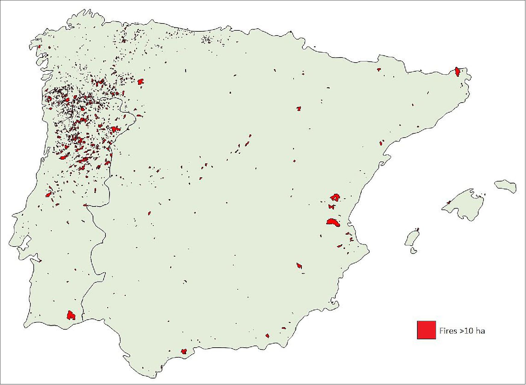
Legend to Figure 35: This image shows all regions on the Iberian Peninsula where fires spreading over an area of more than 10 hectares occurred between 2010 and 2014. The high density of the fires underlines the importance of fire risk protection. The information by the Deputacio Barcelona helps to prevent large areas from burning and protect human lives.
• December 18, 2014: The measurements of salt in surface seawater are crucial for understanding ocean circulation and Earth's water cycle, and ESA's SMOS mission is instrumental in this endeavour. Since its launch in 2009, SMOS has effectively monitored changes in soil moisture and surface seawater salinity, providing the longest continuous record of sea-surface salinity measurements from space. This mission captures the complex interactions of water exchanges among the oceans, atmosphere, and land, revealing how factors like evaporation, precipitation, river discharge, and the melting and freezing of ice influence salinity dynamics. 74)
- Salinity, alongside temperature, plays a significant role in driving ocean circulation, which in turn affects global climate patterns. By delivering comprehensive and continuous data on these essential variables, SMOS enhances our understanding of the water cycle's interactions and supports predictions of climate-related phenomena, establishing itself as a vital resource for researchers and climate scientists alike.
• November 2, 2014: As the SMOS spacecraft marks its fifth anniversary in orbit, it has significantly contributed to our understanding of Earth's water cycle by providing crucial data on soil moisture and ocean salinity. The satellite carries a novel sensor that captures images of "brightness temperature," which relates to the microwave radiation emitted from Earth's surface. This data reveals monthly variations in sea-surface salinity, highlighting significant deviations in the tropical Pacific and Indian Oceans associated with climatic phenomena such as La Niña and the Indian Ocean Dipole. 75) 76)
- In addition to advancing scientific knowledge, SMOS data has practical applications, with 18 TB distributed annually—13 TB for scientific research and 5 TB for near-real-time applications. For instance, the European Centre for Medium-Range Weather Forecasts (ECMWF) integrates these observations to enhance surface air temperature and humidity forecasts, especially in the southern hemisphere where conventional data is scarce. SMOS data also supports applications such as forecasting river runoff, monitoring drought conditions, and predicting crop yields, proving especially valuable in regions with limited ground-based observation networks.
• September 2014: The SMOS mission operations have been officially extended to 2017, as confirmed by both ESA and CNES during their respective reviews. This extension introduces new challenging objectives that emphasize the synergistic scientific exploitation of SMOS data alongside other Earth observation missions such as Aquarius, SMAP, and the Sentinel satellites. Key goals include enhancing the understanding of geophysical phenomena like El Niño and droughts over longer timescales, merging SMOS data with other L-band observations to create long-term datasets and thematic records, as soil moisture and ocean salinity are classified as Essential Climate Variables (ECVs). 77)
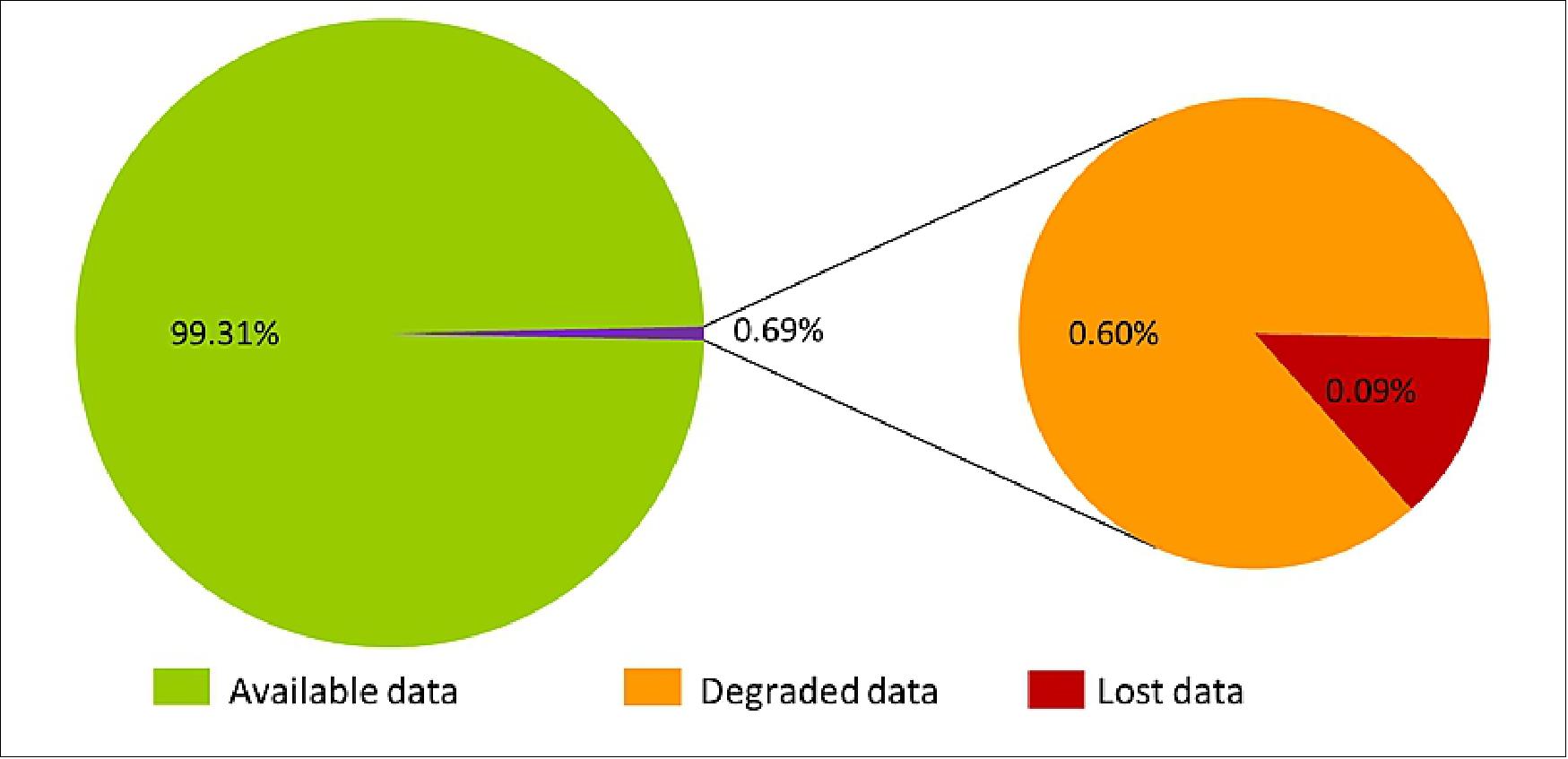
- Currently, the SMOS instrument, MIRAS, continues to operate nominally, with some known onboard anomalies. Since the start of routine operations in May 2010, the cumulative data loss due to instrument unavailability has been minimal, at 0.09%, while degraded data accounts for 1.07%. Additionally, the continuous observation data sets are vital for both operational and scientific users, who have expressed a need for data continuity in (semi-) operational applications following the maturation of SMOS data products.
• July 2014: The SMOS mission continues to deliver essential data on soil moisture and ocean salinity, now extending its operational life until at least 2017 due to its growing versatility and practical applications. In its fifth year on orbit, SMOS has demonstrated its capability to provide accurate measurements of thin sea ice, crucial for weather and climate forecasting. Although originally designed for different purposes, the satellite's ability to detect radiation emitted by ice has enabled it to measure ice thickness down to 50 cm, particularly focusing on younger ice in the Arctic. This information has become increasingly valuable for operational users, leading to the development of new products and services in collaboration with institutions such as the University of Hamburg. 78)
- The extension of SMOS's mission allows for further exploration of innovative scientific applications and enhances potential synergies with other missions. ESA's collaboration with Germany's IRO-2 project aims to create a prototype system for sea-ice forecasting and ship routing, further validating SMOS data. Additionally, the upcoming launch of NASA's SMAP mission and the data from the Copernicus Sentinel missions present opportunities for combining various datasets, such as correlating sea-surface salinity from SMOS with temperature and height information from Sentinel-3. This collaborative approach not only enhances the scientific value of the data but also broadens its practical utility in addressing global challenges.
• May 2014: ESA's SMOS mission has expanded its original focus on understanding the water cycle to include applications in drought prediction and crop yield improvement, particularly in regions vulnerable to famine. The U.S. Department of Agriculture (USDA) leverages satellite images and soil moisture data from SMOS to monitor abnormal weather patterns that could impact crop production. This information contributes to their monthly estimates of global agricultural production, supply, and distribution, providing crucial insights for traders and decision-makers, especially in countries at risk of severe drought. 79)
- By measuring soil moisture in the root zone during the growing season, SMOS helps identify the onset and severity of drought, allowing analysts to forecast crop health and productivity. The USDA has reported positive outcomes from using SMOS data, particularly in southern Africa, where conventional rain gauges are scarce. This enhanced capability has led to the development of new products available on the USDA's Crop Explorer website, further underscoring the mission's versatility and significance in addressing food security challenges. 80)
• May 2014: The Thermal Control Subsystem (TCS) for the MIRAS instrument, comprising 69 single antenna elements, has successfully met stringent thermal requirements essential for the validity of scientific data. The LICEF receivers have maintained an average temperature around 22ºC with minor seasonal variations, meeting the required maximum spatial gradient of 6ºC, although slight exceedances were noted during equinoxes. Additionally, orbital temperature excursions for these receivers remained below 4ºC. However, the NIR antennas experienced significant thermal fluctuations influenced by external conditions, with a cooling effect observed in their temperature ranges over the first eight months of the mission.
- Some anomalies were recorded, such as a temperature jump in the NIR_AB antenna and a permanent failure in the B1 segment of the Y-shaped antenna. In response, alternative thermal control measures were developed, utilizing temperature readings from thermistors to ensure the continuity of operations and maintain data quality. Overall, the TCS has effectively managed thermal conditions to support the scientific objectives of the mission, despite challenges encountered during the operational phase (Ref: 24).
• January 2014: The SMOS mission continues to operate nominally, consistently delivering global soil moisture and ocean salinity data. Notably, the DOME-Cair airborne field campaign, conducted in January 2013 over a 12-day period at the Concordia research station in Antarctica, aimed to validate data from both ESA’s SMOS and GOCE missions. The campaign revealed a remarkable similarity in the spatial patterns observed by the microwave and gravity instruments, highlighting the effectiveness of the SMOS mission in contributing to scientific understanding. 81)
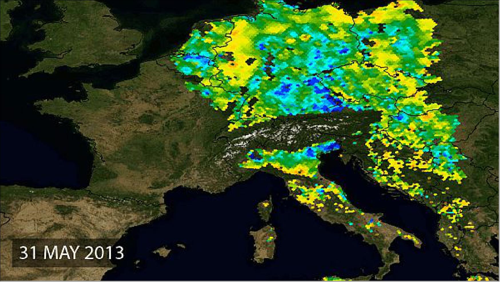
• June 2013: As central Europe faces its most severe floods in centuries, forecasters are looking to ESA’s SMOS satellite to enhance future flood prediction accuracy. SMOS monitors surface soil moisture and the salt concentration in seawater, providing valuable data that helps scientists understand Earth’s water cycle and improve weather forecasts (Figure 37). 82)
- The current flooding has been exacerbated by a wet spring followed by heavy rainfall. Prior to the downpours, SMOS indicated record moisture levels in German soils, reaching their highest levels ever observed. By the end of May, soils were nearly saturated, and additional rainfall caused excess water to run off instead of being absorbed, leading to the devastating floods.
• December 2013: The SMOS instrument, MIRAS, is functioning nominally despite some known onboard anomalies. Since the start of routine operations in May 2010, the cumulative data loss due to instrument unavailability has been 0.11%, while degraded data has reached 1.42%. Importantly, there has been no data loss during the acquisition of MIRAS raw data at ground stations, a success attributed to the implementation of an onboard data recording overlap strategy. 83)
• May 2013: ESA reports that the situation regarding Radio Frequency Interference (RFI) for the SMOS mission is steadily improving, particularly in Europe and North America. This enhancement has significantly boosted the quality of sea surface salinity data collected over the northern hemisphere, especially above 60° latitude. 84)
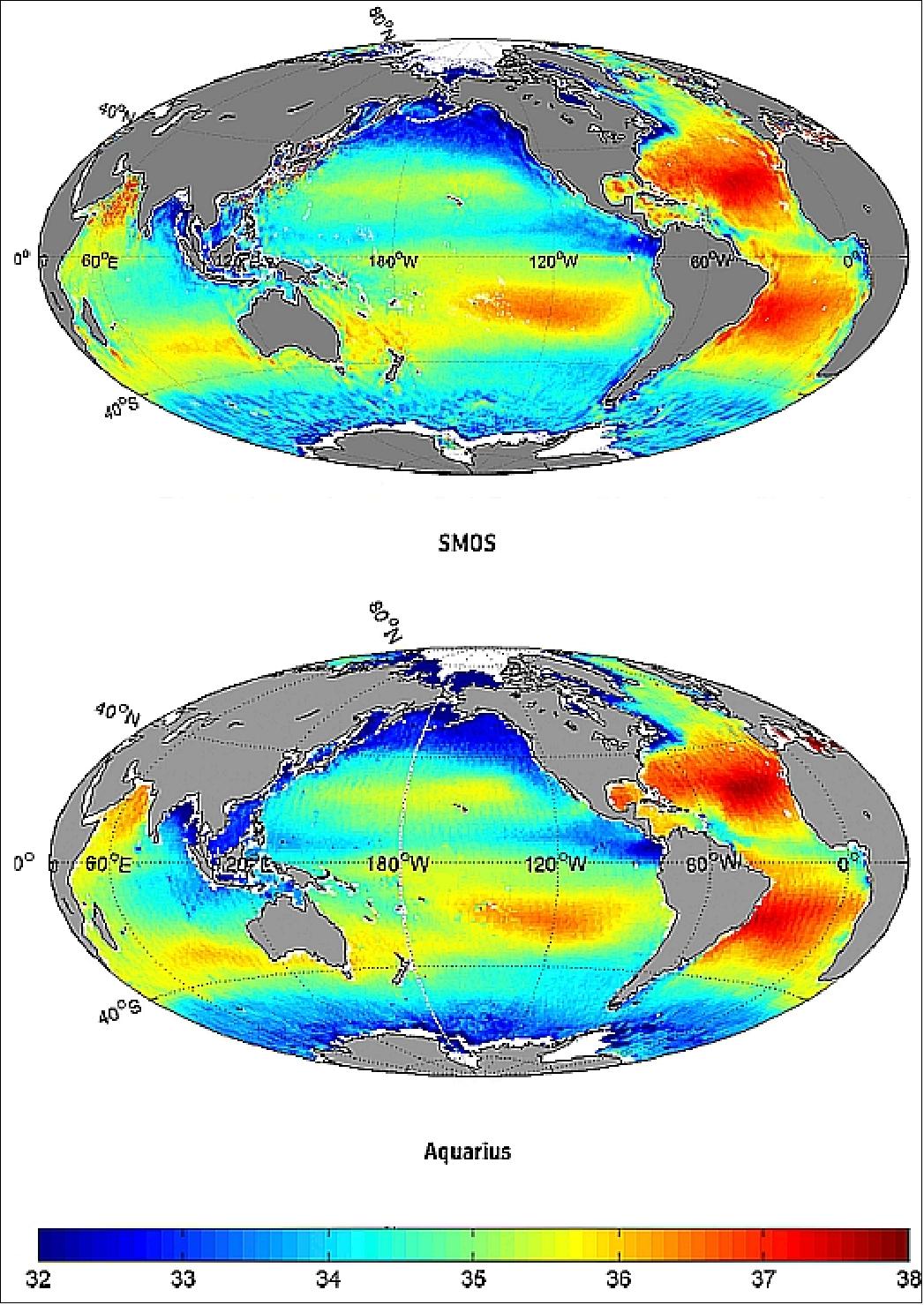
• April 2013: Both ESA’s SMOS and NASA’s Aquarius missions are closely monitoring ocean salinity from space, but with slightly different approaches. By combining their complementary strengths, researchers are advancing climate science. Ocean salinity, which is influenced by the balance between evaporation and precipitation, plays a vital role in Earth's water cycle and ocean circulation, both of which are crucial to regulating climate. As an "essential climate variable," salinity is a key parameter for understanding climate change. 85)
- While both SMOS and Aquarius use L-band radiometers to map ocean salinity, their designs differ (Figure 38). Aquarius provides higher pixel accuracy, whereas SMOS offers more frequent revisit times and better spatial resolution. Although the data from both missions are in agreement, scientists are exploiting these differences to gain deeper insights into ocean salinity variations. The complementary benefits of these missions were a focus at the SMOS & Aquarius Science Workshop in Brest, France, in April 2013. 86)
• February 22, 2013: New findings presented at ESA’s European Space Astronomy Centre (ESAC) reveal that SMOS is offering fresh insights into the dynamics of the Gulf Stream, one of the most closely studied ocean currents. Originating in the Caribbean and flowing toward the North Atlantic, the Gulf Stream plays a crucial role in transferring heat and salt, impacting the climates of the east coast of North America and the west coast of Europe. 87)
- SMOS salinity observations show how warm, salty water from the Gulf Stream meets colder, less-salty water from the Labrador Current off Cape Hatteras, North Carolina. The satellite can track the mixing of these water masses and distinguish the eddies formed when parcels of warm, salty water separate from the Gulf Stream and mix with the colder, fresher waters of the Labrador Current. These insights enhance understanding of ocean circulation and its influence on climate.
• November 2012: At the end of its nominal three-year mission, the SMOS spacecraft and its payload remained in excellent technical condition, allowing the mission to continue providing valuable data beyond its original timeline. SMOS has proven instrumental in offering new data products, supporting applications in oceanographic, meteorological, and hydrological forecasting, as well as climate change research. By measuring microwave radiation emitted from the Earth’s surface, SMOS maps soil moisture and sea surface salinity, both critical for understanding the global water cycle. These measurements, delivered as 2D "brightness temperature" images, are currently utilized in weather and flood forecasting, drought monitoring, and crop yield forecasting, benefiting everyday life and potentially mitigating billions in economic impacts from extreme weather events. 88)
- SMOS data have also opened new avenues for research, such as monitoring the freeze-thaw cycles of soils, which is relevant for tracking permafrost activity and understanding land-atmosphere gas exchanges. Soil moisture data, in particular, are crucial for studying water and energy exchanges between land and the atmosphere, contributing to water resource management, agriculture, and flood prediction. Early studies by ECMWF show that incorporating SMOS-derived soil moisture data improves temperature and humidity forecasts. Additionally, the Finnish Meteorological Institute has used SMOS data to track soil frost depth in northern Europe, offering valuable insights for climate applications, especially regarding the behaviour of permafrost and related gas exchanges. Multi-year SMOS data are expected to further enhance climate modelling and analysis of seasonal and inter-annual variations.
• July 2012: More than a dozen radio signals that interfered with data collection for ESA’s SMOS mission have been switched off. This effort benefits not only SMOS but also NASA’s Aquarius mission, which operates at the same frequency to measure ocean salinity. After the SMOS mission's launch, numerous unlawful signals were detected, rendering some data unusable. ESA has since worked with national authorities to locate and eliminate these sources of interference. 91)
- One of the largest contamination areas was over the North Pacific and Atlantic oceans, mainly from military radars. Now, at least 13 interference sources in northern latitudes have been shut down, significantly improving SMOS observations in these regions. Accurate salinity measurements, previously hindered above 45 degrees latitude, are now possible.
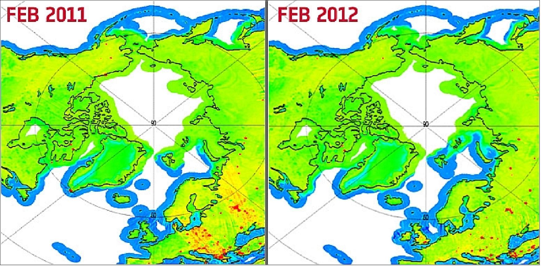
Legend to Figure 39: The two images show the RFI at northern latitudes in February 2011 and February 2012. Several radars are observed (the red ‘dots’, visible because they exceed the natural variability for brightness temperature measurements over land) over Northern Canada and at the southern tip of Greenland. The authorities from Canada and Greenland were informed and requested to take action. Canada started to refurbish their equipment in the autumn of 2011, while Greenland switched off their transmitters in March 2011.
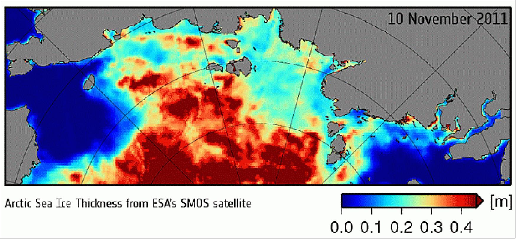
• December 2011: ESA reports that Finnish Meteorological Institute (FMI) scientists are using SMOS data to detect and map frozen soils, allowing not only the extent but also the depth of the frozen layer to be inferred. This adds to the versatility of the SMOS mission, which provides critical data on both soil moisture and ocean salinity. In addition, SMOS can map the thickness of polar sea ice. The University of Hamburg's Institute of Oceanography has developed algorithms to interpret MIRAS instrument data for this purpose. These ice thickness measurements will aid in monitoring seasonal changes and help investigate processes related to Arctic warming 92) 93)
• August 2011: In its first 1.5 years in orbit, the SMOS mission has undergone a steep learning curve, focusing on refining calibration techniques, image reconstruction algorithms, and addressing radio-frequency interference (RFI). The mission is close to meeting its target of 4% accuracy for soil moisture and 0.3-0.5 psu accuracy for sea surface salinity, despite aiming for 0.1 psu. New applications like permafrost monitoring, ice thickness measurements, and hurricane wind observations have been successfully demonstrated. However, further work is required to improve the accuracy of certain parameters and refine image reconstruction and retrieval algorithms. 94)
- The MIRAS instrument's performance has been assessed by comparing brightness temperature images with data from terrestrial radio telescopes, the Pacific Ocean, and Antarctica. While MIRAS generally meets specifications, two issues remain: a systematic error over the ocean caused by antenna pattern and calibration errors, and long-term stability, particularly when measured against ocean or Antarctic models. These discrepancies, partially due to model inaccuracies, need further evaluation. Proposed improvements for future MIRAS missions include a hexagonal array, enhanced thermal design, and increased robustness against RFI, which could significantly improve radiometric accuracy and operational capabilities.
System parameter | Specified Value | Measured Value |
Systematic Error | 1.5 K rms ( B ) | 0.33 K rms (E, sky) |
Level-1 SM Radiometric Sensitivity | 3.5 K rms ( B ) | 2.5 K rms (B, Antarctica) |
Level-1 OS Radiometric Sensitivity | 2.5 K rms ( B ) | 2.0 K rms (B, ocean) |
Short Term Stability | 4.1 K rms ( E ) | 3.5 – 3.8 K rms (E, ocean) |
Long Term Stability | 0.03 K / 2 months | 0.14 K / year (sky) |
Pointing | 400 m | 221 m (ascending orbit) |
• February 7, 2011: After resolving the onboard anomaly experienced by the MIRAS instrument on December 31, 2010, nominal operations resumed on January 12. Following this, recalibration activities were successfully completed, and nominal data quality was fully restored on February 7, 2011, at 09:40 UTC. 96)
• January 24, 2011: Following the anomaly related to the anomalous temperature readings in one segment of antenna arm B, the SMOS instrument MIRAS is now back to nominal operations as of 12 January 2011. To return to nominal data production re-calibration activities are necessary to ensure the quality of the SMOS data delivered to the user, which are presently performed and assessed. 97)
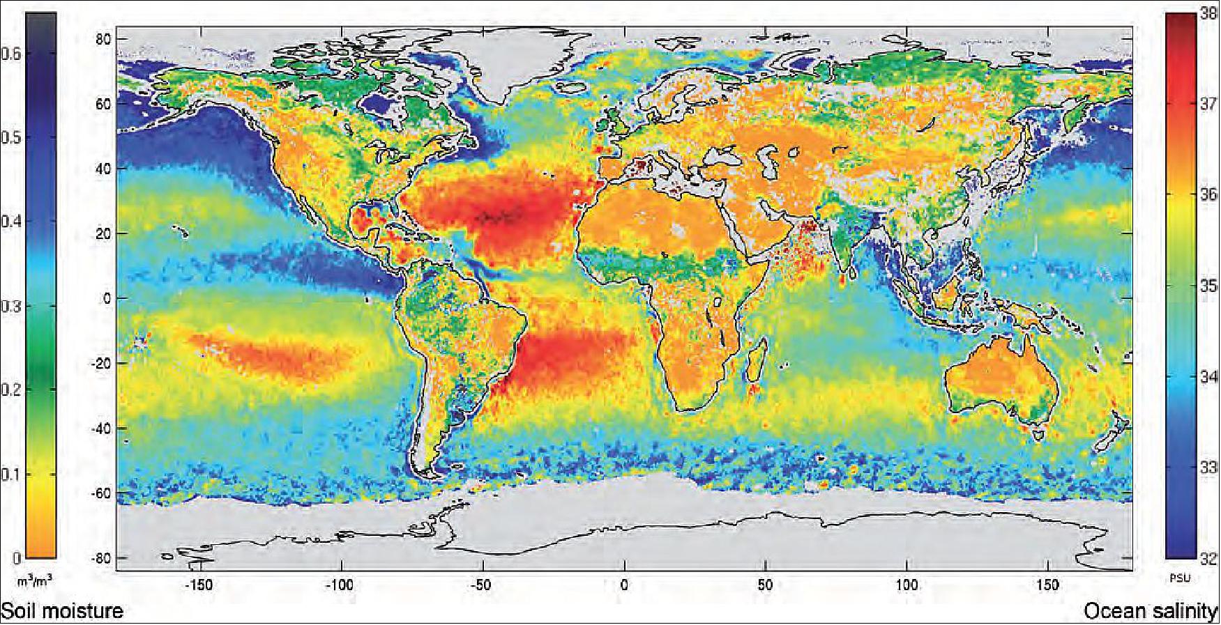
• November 2, 2010: SMOS celebrated its first year on orbit. All data (brightness temperatures (level-1) and soil moisture and ocean salinity data (level-2)) have been released to the science community at large. The first global map of both soil moisture and ocean salinity was delivered by the SMOS Earth Explorer. By consistently mapping soil moisture and ocean salinity, SMOS is advancing our understanding of the exchange processes between Earth's surface and atmosphere and also helping to improve weather and climate models. 98) 99)
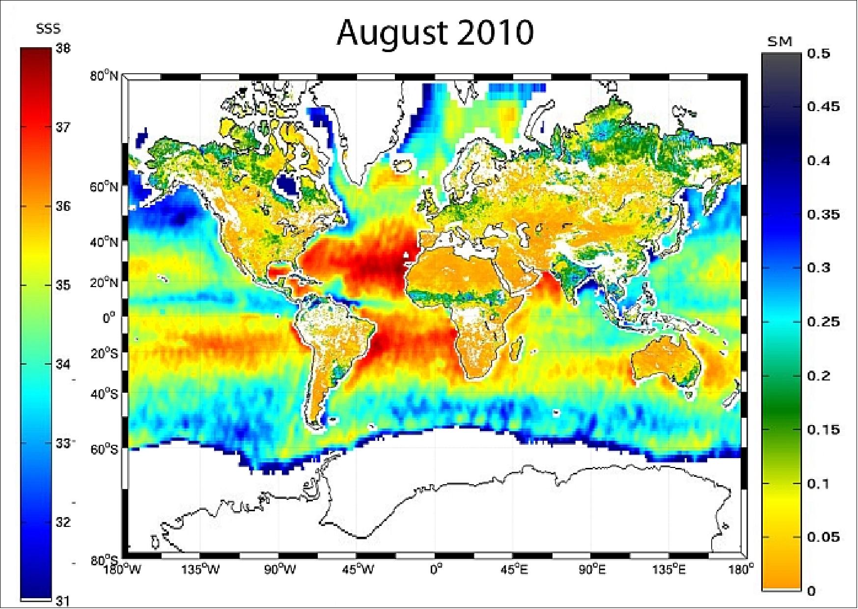
Legend to Figure 40: For the first time, data on soil moisture and sea-surface salinity have been combined on one map. The map was generated by combining global measurements acquired in August 2010. The SSS data have a spatial resolution of 1º x 1º. Comparison with in situ measurements in the oceans averaged over 1º x 1º in August reveals a quasi-global accuracy of 0.4 practical salinity units, which is very promising after just one year in orbit.
• October 2010: The SMOS mission has delivered impressive results, but the MIRAS instrument, which operates in the protected L-band (1400-1427 MHz), has faced significant interference from radar, TV, and radio transmissions. These unwanted signals, violating the ITU-protected band, have occasionally contaminated the data, particularly in regions like southern Europe, Asia, the Middle East, and some coastal zones, making parts of the data unusable. Despite this, SMOS has met its scientific goals in areas free from RFI. 100) 101) 102)
- To maximize the mission's effectiveness, ESA has worked to address the RFI issue through international collaboration. TV transmitters, radio links, security networks, and terrestrial radars were identified as the main sources of interference. ESA has been engaging in the complex process of shutting down illegal transmissions and reducing excessive out-of-band emissions to improve data quality.
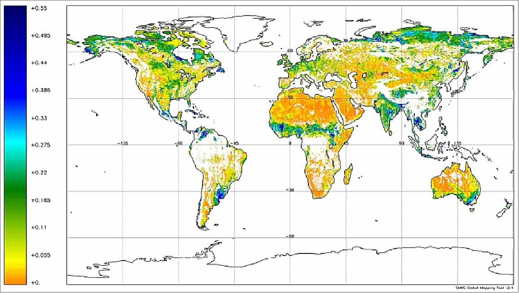
• July 2010: The SMOS mission provides observations of "brightness temperature," which measures radiation emitted from the Earth's surface. This data enables the creation of global soil moisture maps every three days and ocean salinity maps at least once every 30 days. 104)
• May 21, 2010: ESA's SMOS satellite completed its six-month commissioning and formally began operational life. This milestone means the mission is now set to provide much-needed global images of soil moisture and ocean salinity to improve our understanding of the water cycle. 105)
• April 2010: The HUT-2D, a 1.41 GHz interferometric radiometer developed by Aalto University, was used to measure three SMOS validation target areas: one in Denmark and two in Germany. Alongside the HUT-2D, the EMIRAD radiometer from the Technical University of Denmark, with two fully polarized receivers, was installed on a research aircraft for the study. The test sites included the Upper Danube Catchment (UDC) in Southern Germany, covering 77,000 km² of agricultural land, the Rur Erft Catchment (REC) near Aachen, spanning the Belgian-Dutch-German border, and the Skjern River catchment in Western Denmark, covering 2,500 km² near the coast. 106)
• February 2010: in less than four months since launch, the first calibrated images are being delivered by ESA’s SMOS mission. These images of 'brightness temperature' translate into clear information on global variations of soil moisture and ocean salinity to advance our understanding of the water cycle. Since its launch on Nov. 2, 2009, engineers and scientists from various institutes in Europe have been busy commissioning the SMOS satellite and instrument. This commissioning phase, which will continue until the end of April, initially involved testing the Proteus platform – a generic 'satellite bus' developed by the French space agency CNES and Thales Alenia Space – and the all-important MIRAS instrument developed by EADS-CASA in Spain under contract to ESA. Both platform and instrument have shown excellent performance during their first four months in orbit. 107)
• December 2009: SMOS successfully completed its Launch and Early Orbit Phase (LEOP), confirming that all systems are functioning properly and the satellite is ready for full commissioning. The MIRAS instrument is now undergoing necessary calibrations to ensure optimal data quality. Calibration and data processor adjustments are ongoing, with the first routine processed data expected to be shared with the calibration/validation team by March 2010. Initial analysis of the data reveals significant radio frequency interference within the protected band, which is typically reserved for radio astronomy and passive remote sensing (Ref. 110)
• November 17, 2009: The MIRAS instrument was activated, and is functioning as expected, with all key subsystems, such as the receivers, optical fibers, and correlator unit, working flawlessly. Following the successful launch and early orbit phase, engineers are now focusing on evaluating the downlink quality and calibrating the instrument. 108)
• November 2, 2009: CNES, responsible for operating the satellite, confirmed that the MIRAS instrument’s three antenna arms have deployed as planned and that the instrument is in good health. 109)
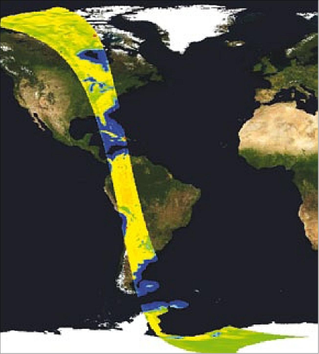
Sensor Complement
MIRAS (Microwave Imaging Radiometer using Aperture Synthesis)
MIRAS was developed by the prime contractor EADS-CASA Espacio, Madrid, Spain. The SMOS sensor assembly (the only instrument of the PLM) is a dual polarized 2-D interferometer operating at L-band (1.41 GHz) and based on the MIRAS concept of several airborne campaigns (Note: in 2004 the name MIRAS was also adopted for the instrument on the SMOS spacecraft).
The overall objective of MIRAS is to provide records of pixel brightness temperatures over incidence angles from 0º up to 55º across a 900 km swath, with a spatial resolution in the range of 30-50 km. From these profiles and auxiliary information, like surface physical temperature, roughness and ionospheric total electron content among others, soil moisture and sea surface salinity will be retrieved.
The design of the passive spaceborne instrument uses three coplanar arms consisting of an elementary antenna regularly spaced (0.875 λ, maximum redundancy) in a Y-shaped configuration (also referred to as a sparsely populated antenna, a thinned array is substituted for a filled array, each deployable antenna arm has a length of 4 m). In this concept, an interferometric Fourier synthesis is applied to derive images from the correlations between each pair of antenna elements (small independent receivers) operating in the microwave region. The 2-D SMOS interferometer permits the brightness temperature to be measured simultaneously at different incidences, and at two polarizations. Moreover, the instrument records an entire scene instantaneously. As the S/C moves, a given point within the 2-D FOV is observed from different view angles. A series of independent measurements is obtained permitting the derivation of surface parameters with improved accuracy. The brightness temperature field of such a design is reconstructed with a resolution corresponding to the spacing between the outmost receivers. 111) 112) 113) 114) 115) 116) 117) 118) 119) 120) 121)
MIRAS, operating at L-band (1.4-1.427 GHz, or 21 cm wavelength), employs a Y-shaped antenna arrangement, consisting of three arms, separated at 120º. Every antenna arm supports a row of evenly spaced receivers along its span. Each arm consists of three deployable segments.
There are 69 antenna elements - the so-called LICEF (Lightweight Cost-Effective Front-end) receivers -, which are equally distributed over the three arms and the central structure (hub). Each LICEF is an antenna-receiver integrated unit (four-probe patch antenna with a combiner/polarization circuit) that measures the radiation emitted from the Earth at L-band (1404-1423 MHz). The LICEF units are built by MIER Comunicaciones SA, Barcelona, Spain, and include a dual-polarized antenna and a critical bandpass filter.
Each LICEF measures the thermal noise emitted by the Earth in the L-band by means of a complex amplification chain and filtering in RF and IF comprised of MMIC (Monolithic Microwave Integrated Circuit) for reducing consumption and weight. The result is a 1 or a 0 quantization of the in-phase and quadrature components of the received signal, depending upon the noise uptake level. LICEF is a highly frequency-selective receiver that avoids capturing disturbing signals from adjacent bands that would corrupt the noise sought from earth for measurement. 122) 123)
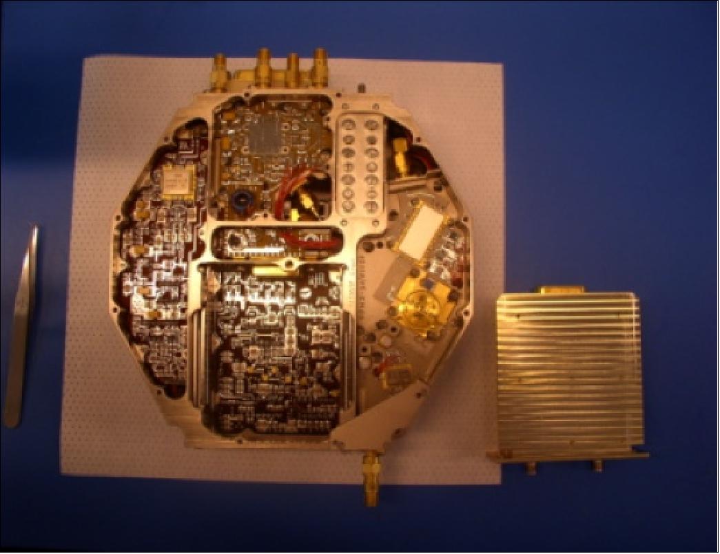
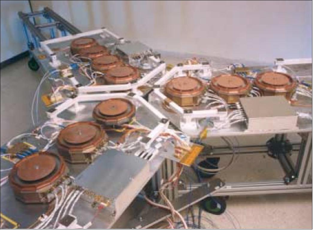
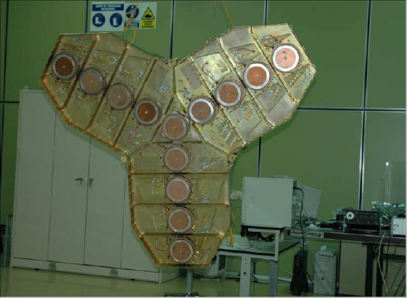
The total deployed arm length is about 4 m. The hub interfaces with the platform and houses some common equipment, such as a total-power radiometer for absolute calibration. The instrument structure (modular design) uses CFRP (Carbon Fiber Reinforced Plastic) material for reasons of stiffness. Each receiver can be commanded to measure either H and V polarization, or an internal load. The calibration network (subsystem) enables correlative measurements for the entire array.
It consists of the following elements (noise sources that are being fed into the receivers):
• A central redundant noise diode, distributed to all receivers of the hub
• Distributed noise diodes on each arm segment; this allows measurements not only of the segment receivers but also of the adjacent ones on either side of the hub or the next element.
Furthermore, three NIR (Noise Injection Radiometer) at the hub are measuring the H and V polarization simultaneously to enable the “zeroth baseline” correlation. All individual receivers digitize the measured I and Q signals and send them, via a point-to-point optical fibre connection, to DICOS (Digital Correlator System), in which the correlations between all possible receiver pairs are made and accumulated for the duration of the integration period (1.2 s). The calibration frequency depends on the thermal gradient and the receiver behaviour with the temperature. The operating temperature of MIRAS is kept within a range of 0 to 50ºC. 124)
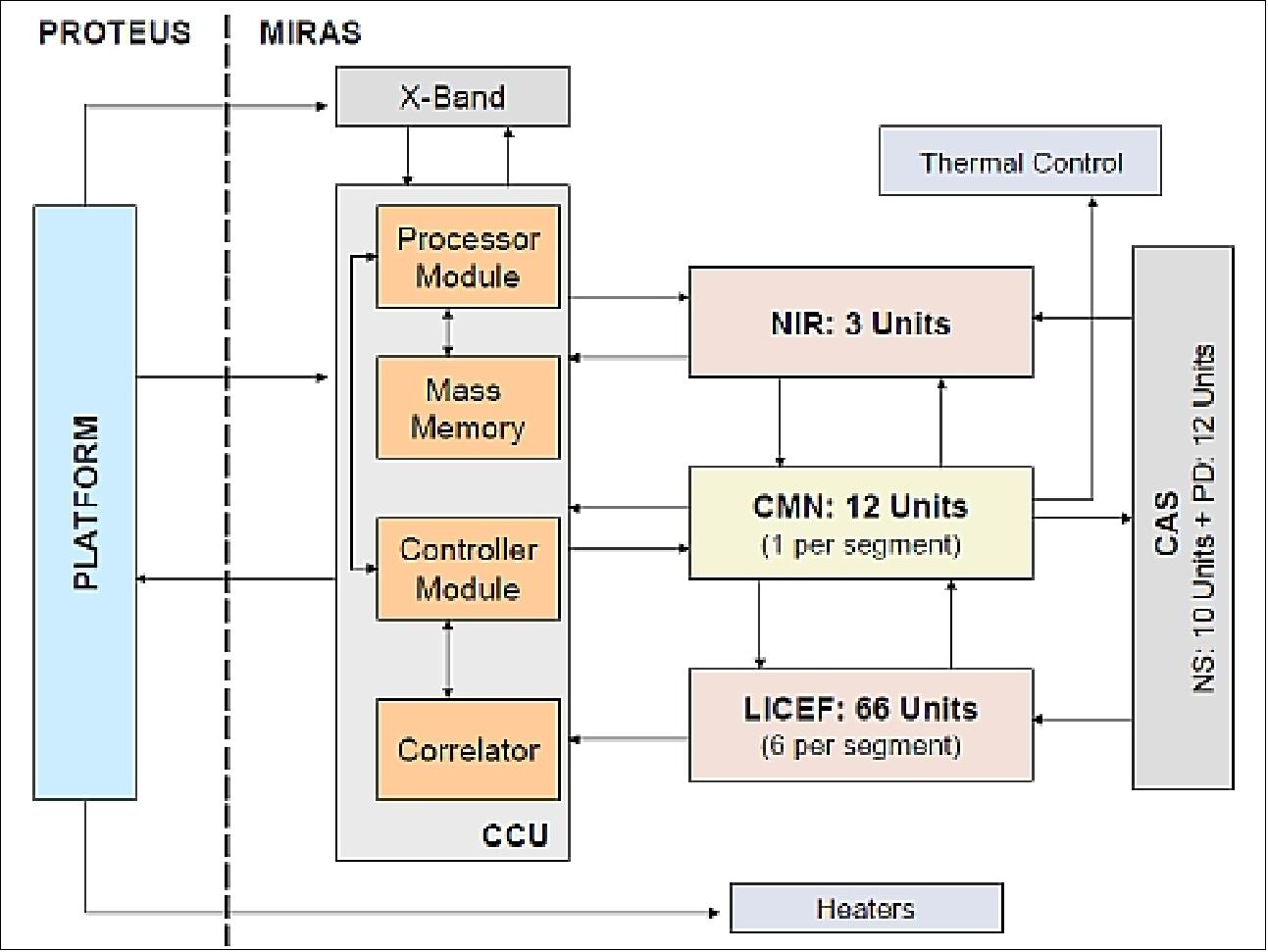
Background on L-band radiometry: Operating the radiometer in the L-band provides the maximum sensitivity of the emissivity to both SM (Soil Moisture) and OS (Ocean Salinity). However, it implies antenna diameters of several meters in order to meet the spatial resolution requirement for SM mapping which, for the design of SMOS, has been set at 50 km. A large real-aperture antenna on an LEO satellite poses a number of practical difficulties. A problem also arises from the need to achieve global coverage of the Earth within three days, which implies a large instrument swath. Microwave imaging by aperture synthesis provides an effective alternative to more classical solutions like the use of mechanically or electrically steered antennas and pushbroom instruments. This interferometric approach to microwave radiometry, inspired by the techniques developed in radio-astronomy over several decades, is based on the use of many small antenna/receiver units, geometrically arranged so as to sample the signal that would have been received by a real-aperture antenna. This sampling in the spatial domain, enabled by the use of multiple antenna elements, provides a scanning capability through a wide swath by means of (ground) signal processing only. 126) 127)
Background on main instrument characteristics of MIRAS: Each antenna/receiver unit is based on a patch antenna without a dielectric substrate with about 70º half-power beamwidth, a directivity of about 8 dB and provides both H and V polarizations with excellent cross-polarization characteristics (co-polarization/cross-polarization ratio > 25 dB). A single receiver chain per antenna element is available, so each unit can operate on either H or V polarization upon command from a control unit. In each receiver, the antenna signal is filtered to the selected bandwidth (1404 to 1423 MHz, in a region of the spectrum reserved for passive measurements), amplified and finally sampled and converted to a 1-bit digital signal. The MIRAS output data stream, combining both I and Q components at a rate of about 130 Mbit/s, is transmitted to the correlator unit by means of an optical fibre link. Each element also receives (via a second optical fibre link) a centrally-generated reference clock signal in order to perform the frequency down-conversion and the sampling with phase coherence among all elements. An oversampling by a factor of about 2 with respect to the Nyquist criterion is achieved in each receiver, which improves the radiometric sensitivity. In the correlator unit, after conversion from optical to electrical signals, a massive bank of 1-bit/2-level correlators implemented in dedicated integrated circuits performs the cross-correlations between all signals. Horizontal and vertical polarization images are interlaced and the cross-correlation for each polarization is performed over a 0.3 s period. Up to 5 images are then averaged, so two images (one per polarization) are available every 3 s.
Each antenna arm provides 3 x 6 receivers with a polarization capability in H+V. The antenna features four balanced feeds to obtain a co/crosspolarized ratio >25 dB over an angular extension of ±30º.; there is also an intermediate stage for E- and H-radiation pattern alignment. Each receiver outputs the I- and Q-digitized signals. Each receiver is furnished with a suitable filter to reject interference from adjacent bands and to shape the frequency response. A multiplexer converts the eight parallel I- and Q-level bit streams from each group of four receivers into a ten-bit serial data stream (quantization) which is fed into a central demultiplexer for serial/parallel conversion. The digital correlator, at the end of the processing chain, performs a complex correlation (at zero delays) between each pair of antenna elements of the interferometric array, resulting in the so-called “visibility function” at the spatial frequency defined by that particular antenna element baseline. The visibility function is ideally the Fourier transform of the brightness temperature of the scene, weighed by the element gain pattern, and recovered by the inverse Fourier transform. The output is the visibility map.
A typical MIRAS receiver includes the following elements:
1) RF device (with an input switch, a filter and an amplifier),
2) a phase/quadrature frequency down converter,
3) two two-level quantizers and samplers.
The RF bandwidth is limited to 1400-1427 MHz, the input RF filter band is fixed at 1404-1423 MHz (interference avoidance). The I (In-phase) and Q (Quadrature) outputs of all receivers are processed by a matrix of 1-bit digital correlators, located in the hub. 128)
The MIRAS configuration provides a FOV (swath) of about 900 km (the FOV has a hexagon-like shape at an orbital altitude of 763 km, sufficient for a 3-day equatorial revisit time. The antenna boresight is tilted at an incidence angle of 32.5º in the forward along-track direction for nominal radiative flux observations. The instrument tilt maximizes the footprint area for a given resolution goal and antenna spacing ratio. The tilted antenna footprint is represented by the sum of the overlapping individual antenna receivers, each representing a pixel of a distorted hexagon shape with curved sides; all pixel projections are of various sizes and incidence angles.
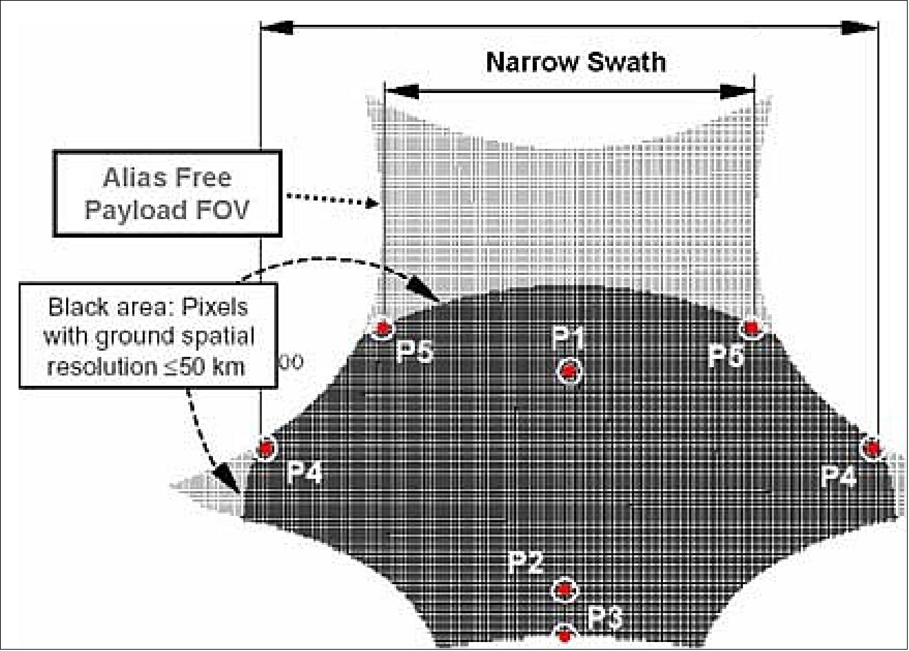
A snapshot brightness temperature map of the FOV is taken every 0.3 seconds with an average resolution of about 5 K over 200 K. Due to the platform motion in orbit, each pixel is measured several times with different spatial and radiometric resolutions and incidence angles. The minimum FOV along-track dimension is about 800 km, this corresponds to 380 snapshots at 0.3 s each. Ground data processing must account for all observation variations in size, shape, angles, overlapping conditions, weighing and averaging schemes, etc., resulting eventually in a brightness temperature map for each snapshot as well as for the accumulated and averaged along-track observation incidences within FOV. The repetitive measurement scheme of radiation, from varying footprints and incidences, has a similar summation effect on the retrieval of the overall signal, as a TDI (Time Delay Integration) scheme for an optical imager.
The overall instrument mass is 369 kg, power ~ 375 W. MIRAS data processing requires the introduction of corrections due to atmospheric, ionospheric, and galactic effects over ocean surfaces. In addition, SSS retrieval requires knowledge of sea surface temperature and sea roughness. For observations over land surfaces, knowledge of the surface temperature is needed with an accuracy of 2 K. These reference parameters have to be obtained from instruments of other missions.
Parameter | Desired | Acceptable | |
Soil Moisture (SM) | SSS (Sea Surface Salinity) | ||
Coverage | Global (separate) | Global | Global (separate) |
Mission duration | 3-5 years | 3-5 years | 3 years |
Frequency | L-band | L+C-Band | L-band |
Polarization | H+V | - | H+V |
Spatial resolution | 10 km | 20 km | 50 km |
Revisit time | 1-3 days | 1-10 days | 3 days |
Radiometric accuracy | 1 K | 0.5 K | 2 K |
Radiometric sensitivity | 1 K | 0.25 K | 3 K |
MIRAS instrument command and data handling. The ICU (Instrument Control Unit) interfaces with the MIL-STD-1553B bus of the S/C. The S/C time signal is used to generate time stamps for the science data, generated and packetized in DICOS. The ICU interfaces with the receivers and the calibration network via CMN (Command and Monitoring Nodes), located on the hub of each arm segment.
The CMN provides a number of functions:
1) switching of receivers and calibration network,
2) acquiring some housekeeping information,
3) providing some power conversion and distribution to the receivers,
4) providing the receivers with a local oscillator signal derived from DICOS.
The MIRAS instrument has three main operational modes:
• Dual-polarization mode, in which all receivers are switched synchronously to either H or V polarization
• Full polarimetric mode, in which segments of the array are switched according to a predefined sequence between H and V
• Calibration modes, in which measurements of the internal load, the noise diodes, or the so-called “fringe washing function” are determined.
Note: After the commissioning phase, one of the two operational modes (dual-polarization or full-polarimetric) will be selected and from that point onwards, MIRAS will be operated in the selected mode.
In-orbit Calibration
MIRAS has two types of in-orbit calibration:
1) external, in which the instrument makes a maneuver to point to the cold sky,
2) internal, in which noise is injected to the receivers.
This one in turn has two modes, one of short duration carried out periodically interspersed with scene measurements, and the other lasting a full orbit and used to obtain the more stable parameters and the sensitivity of all parameters with temperature. 129) 130)
Calibration mode | Type | Objectives |
Sky view | External | - NIR absolute calibration: |
Long calibration | Internal | - U-noise injection (Visibility offset) |
Short calibration | Internal | C-noise injection: |
Selfcalibration | Internal | Calculation of normalized complex correlations |
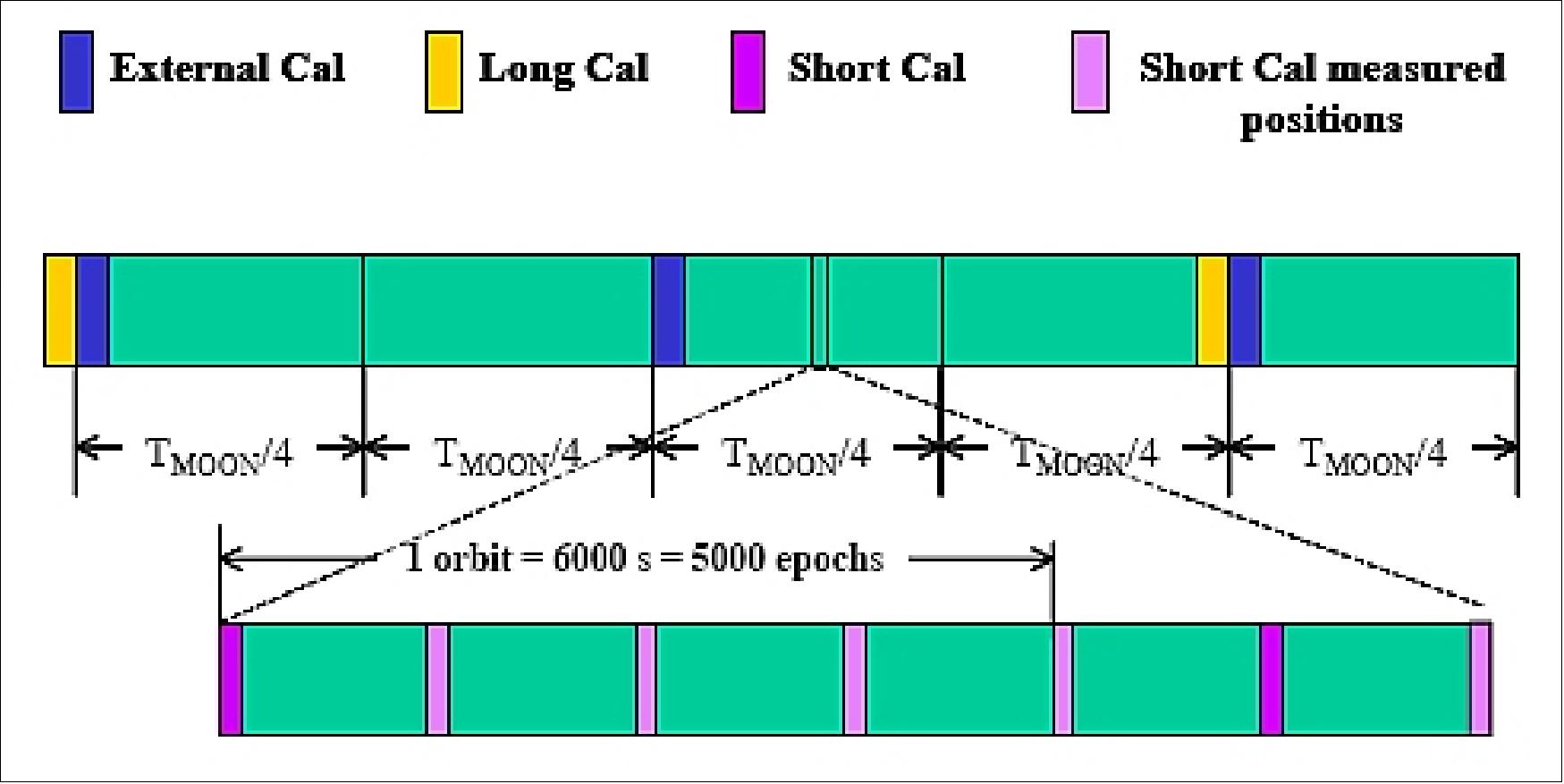
Internal calibration is based on periodically injecting noise to all receivers via dedicated input switches. Due to the difficulty of making a large noise distribution network, a distributed noise approach is used for large baselines. Internal calibration also includes a so-called selfcalibration mode that is used for automatically correcting samplers offset and quadrature error 131)
External calibration: Part of an orbit is devoted to observing the sky to complete the in-orbit calibration, in particular those parameters that cannot be properly calibrated by internal calibration. They are the following: NIR units, Deviations in the antenna patterns and Parametric G-matrix. In one month there will be two identical external calibration events every two weeks. The calibration is carried out by observing an external target selected in the sky in an inertial attitude for part of the orbit.
Internal calibration: Various onboard means are provided to measure the accuracy and stability of the payload data.
These are:
• Matched loads in each of the receivers
• Centralized noise source/network on the hub
• Distributed noise sources/networks in the arms
• Fringe wash function in the CCU (Correlator and Control Unit)
In all calibration activities, the antenna proper is not involved; this represents the “unknown” factors. Therefore, provisions have been made to perform “external” calibrations, by pointing the entire spacecraft to specific targets: either to deep space, the moon, the sun, or known ground targets.
The LICEF (Lightweight Cost-Effective Front-end) receiver parameters of MIRAS are sensitive to temperature and ageing. Hence, they need to be calibrated in flight to ensure that the accuracy requirements of the mission can be met.
For this purpose MIRAS has been provided with:
1) 3 accurate NIR (Noise Injection Radiometer) subsystems as reference radiometers
2) An onboard CAS (Calibration Subsystem)
Both subsystems were developed by Ylinen Electronics (Finland) and HUT (Helsinki University of Technology) or TKK, Helsinki, Finland - as subcontractors to EADS-CASA Espacio of Spain.
The CAS device of MIRAS includes a total of ten Noise Source (NS) units, twelve two-to-six Power Divider units (PD), and interconnecting RF cables. CAS forms a noise distribution network that generates and distributes correlated noise to all the receivers of MIRAS at two different noise levels (hot and warm). There are two different configurations of NS units; each of the arm segments has an ANS (Arm Noise Source) connected to adjacent PD units from two outputs (Figure 47). The hub section (Figure 48), has one HNS (Hub Noise Source). The HNS has three outputs, which are connected to three PD units on the hub. 132) 133) 134)
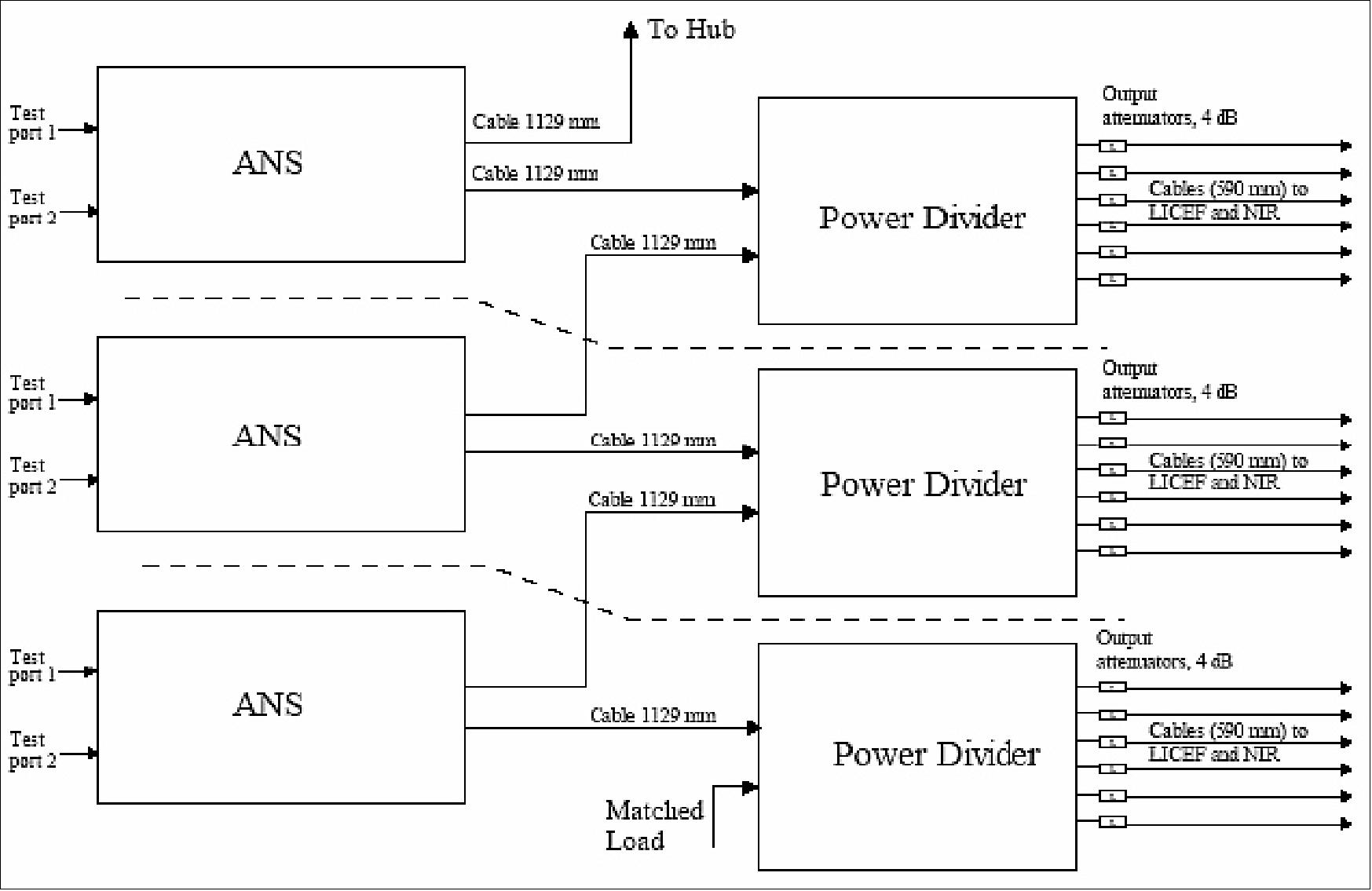
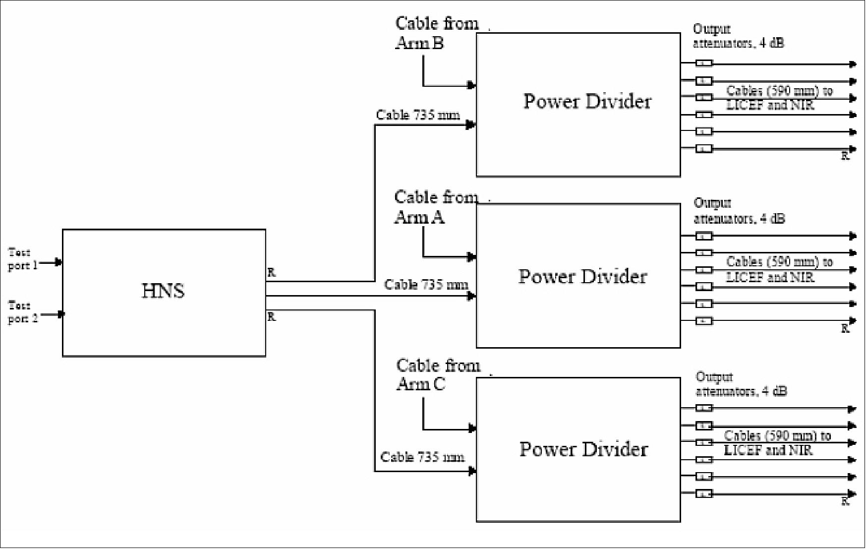
The configuration of the noise distribution network enables each individual radiometer receiver to be fed by two different NS units. The overlapping scheme enables to keep track of the signal over the whole calibration network and thus, establishes a relationship between phase and amplitude among the receivers. The three NIR units are used as absolute reference. The distributed noise generation concept is adopted due to mass and volume constraints of the satellite payload; centralized noise generation (using a single noise source and sufficient division) would require a much larger cable harness.
The block diagram of one HNS is presented in Figure 49. The ANS units are identical with the exception that one of the three outputs is internally terminated. Test ports 1 and 2 are being used on-ground to characterize the relative attenuation and phase differences between the output ports of a NS unit.
Using the RF switches, three distinct noise temperature levels can be generated at the NS output; hot level (approx. 65000 K), warm level (approx. 5000 K), and ambient. Reduced to the output of the CAS subsystem (i.e., the input of individual receivers), the correlated noise levels (thermal noise subtracted) are approximately 1200, 75 and 0 K, respectively.
One ANS device is shown in Figure 50 HNS is otherwise identical to ANS, but it has three outputs instead of two. The mass of the units is approx. 135 g, 295 g and 300 g for PD, ANS, and HNS, respectively. The dimensions of PD and NS units are 95 mm x 57 mm and 85 mm x 115 mm, respectively, not including mounting feet and connectors.
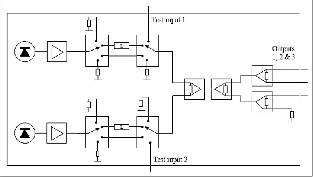
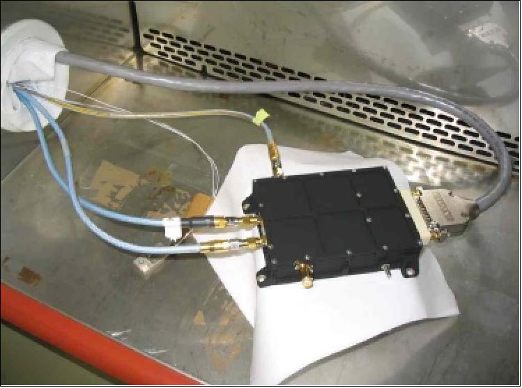
The NIR (Noise Injection Radiometer) subsystem, which consists of three NIR units, works as part of the MIRAS instrument.
The main objectives of NIR are: 135)
• To provide precise measurements of the average brightness temperature scene for absolute calibration of the MIRAS image map
• To measure the noise temperature level of the internal active calibration source for individual receiver calibration CAS (Calibration Subsystem).
• To form interferometer baselines with the regular receivers units in the MIRAS array (so-called mixed baselines).
The NIR performance is of great importance to the SMOS mission.
The measurement challenges are based on the following scenario:
- There is only one accurate external target (cold sky)
- The individual antennas have a wide field of view
- The temperature of the NIR is not actively stabilized varying about 1.5º C per orbit
- Certain calibration parameters cannot be measured on orbit, but on ground only.
The NIR instrument consists of:
• Two radiometer receivers, one for vertical and one for horizontal polarization. The NIR receivers, manufactured by MIER Telecomunicaciones, Spain, are almost identical to the regular LICEF receivers of MIRAS.
• A controller. The controller incorporates an antenna that receives the target noise (Figure ).
• Four-phase stable low-loss RF cables that connect the controller to the receivers.
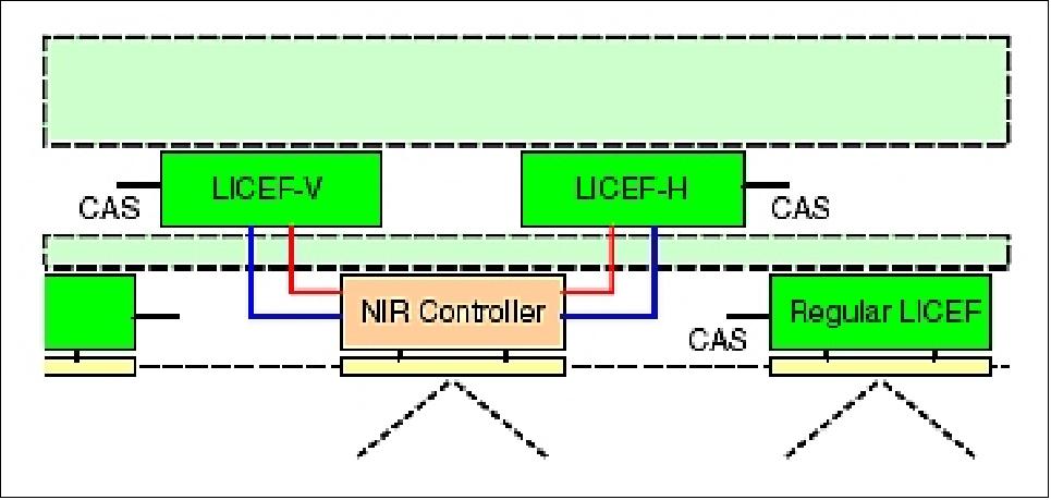
The functions of the controller are to:
a) inject reference noise into the two receiver chains,
b) regulate the amount of the injected noise to keep the system balanced with antenna temperature or with the calibration noise from CAS,
c) control the switches of NIR (Dicke-switches of the receivers and the noise switches of the controller) according to the selected operation mode.
The NIR subsystem has several operational modes for measuring the antenna and CAS noise temperature and for calibration. The antenna temperature is measured using a noise injection mode called the NIR-A mode, and the CAS noise level is measured using a noise injection mode called the NIR-R mode. Also, total power modes are used, for example, to solve the receiver noise temperature.
The NIR calibration approach includes two steps:
1) certain parameters are characterized on-ground,
2) these parameters are applied during orbital calibration, which is carried out frequently.
The in-orbit calibration is based on the measurement of the cold sky, which has a well-known brightness temperature level.
The following parameters were solved during on-ground characterization:
1) antenna and front-end loss,
2) the phase imbalance of antenna and front-end,
3) non-linearity correction,
4) the temperature dependency of noise injection level.
The measured performance meets the requirements set for the NIR subsystem of SMOS. The retrieved ground calibration parameters will be applied during in-orbit calibration when the level of the noise injection, receiver noise temperature and phase imbalance of the channels are solved. After this, the correction for the non-linearity is applied to the measured level of brightness temperature.
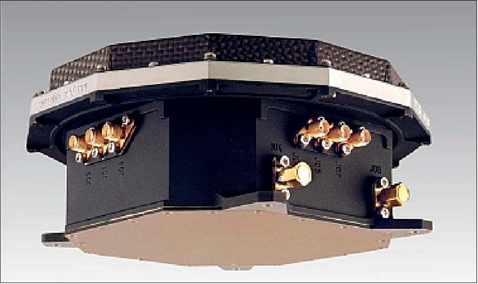
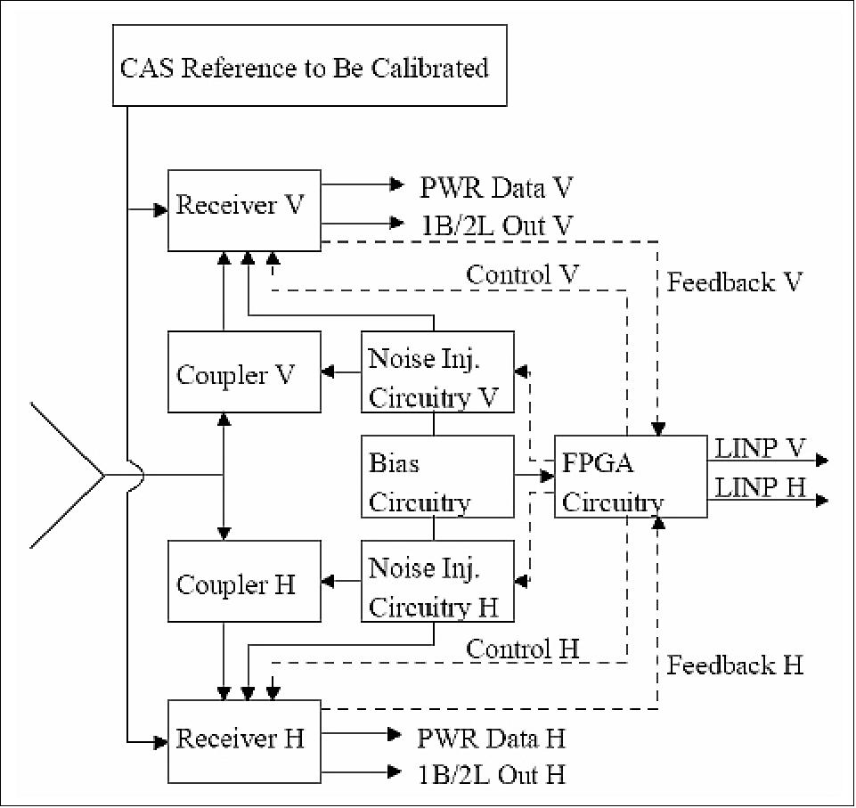
MIRAS (Microwave Imaging Radiometer with Aperture Synthesis) Technology Development
The MIRAS instrument technology development represents a rather complex program of ESA research and validation activities over an extended period which started in1997 with feasibility studies (in 2000 the SMOS Phase-A definition of a space-borne mission was superimposed on this framework effecting in turn the layout of the MIRAS instrument) and is documented in the following reference. Only a few items are mentioned here. 136) 137)
In 1998, ESA started MDPP-1 (MIRAS Demonstrator Pilot Project-1) to provide a technology solution to the inherent challenges of L-band radiometry. The initial objective was to build a representative element of the MIRAS instrument (one entire segment of the arm) to test the technology of a distributed system. This activity was performed by EADS-CASA (Spain) and ended in Oct. 2002 with all critical areas of technology validated.
The MDPP-1 included:
• The SMOS parametric mission design
• The STM (Structure and Mechanisms) for a complete segment, including a deployment mechanism
• Four LICEF (Lightweight Cost-Effective Front-end) antenna receivers. Each LICEF is an antenna-received integrated unit that measures the radiation emitted from Earth at L-band.
• The CAS (Onboard Calibration System) to service one entire segment and the complete hub
• The MOHA (MIRAS Optical Harness) to service one entire segment of the hub. MOHA employs the IEEE 1393-1999 SFODB (Spaceborne Fiber Optic Data Bus), a redundant, cross-strapped, ring-based configuration to provide the following services/functions:
- Connection of the radiometer receivers to the central correlation unit in a star topology
- Synchronous, one-directional data transmission at 112 Mbit/s data rate
- 1300 nm laser diode transmitter and InGaAs PIN photodiode receiver
Note: MIRAS is the first satellite payload to rely critically on fiber optics communications. There are 144 links at 110 Mbit/s (72 to and 72 from the antenna elements). Typical characteristics of the fiber optics implementation are:
- very low EM emission levels (from Tx/Rx)
- galvanic isolation
- mechanically flexible and lightweight
- better phase stability when bent.
In 2000, a parallel and follow-on activity was started at ESA, referred to as MDPP-2, with the objective to demonstrate the following critical aspects of the program:
• A deployment demonstration test for one complete arm of MIRAS (three segments)
• An image validation test using a 12-LICEF MIRAS array.
• Proof-of-concept activities involving: 1) a NIR (Noise-Injection Radiometer), 2) an advanced DISCOS-2 (Digital Correlator System-2), and 3) an advanced BPF-2 (Band-Pass Filter-2)
• The breadboarding of MOHA-3, the optical harness from SMOS Phase-A.
The end of MDPP-2 was in the fall of 2003.
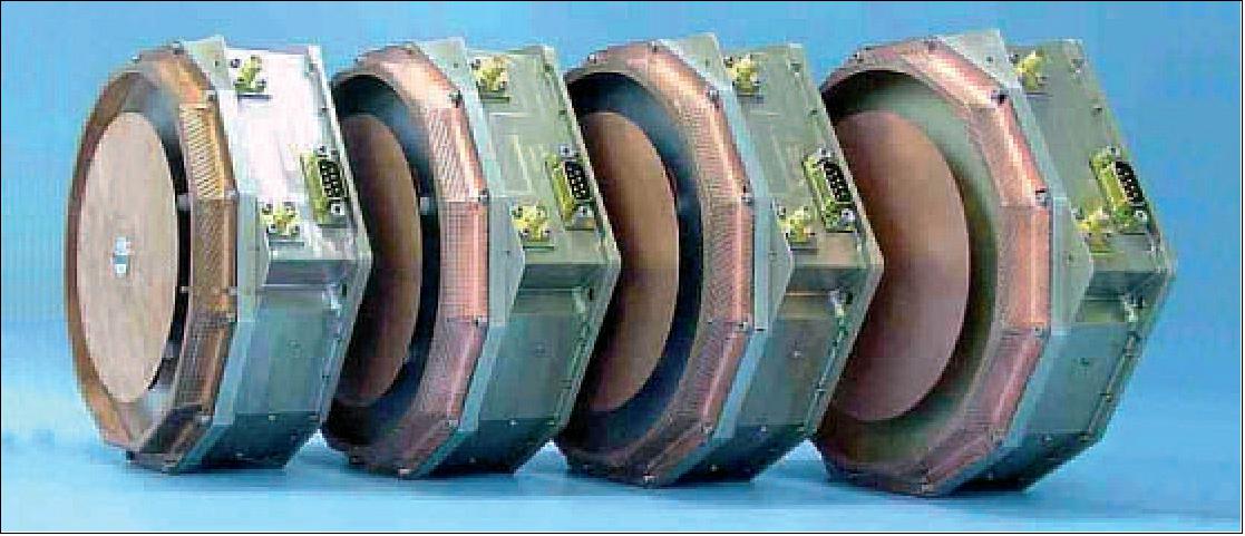
MOHA: The connections between the various elements of the instrument are performed with an optical fiber digital network called MOHA (MIRAS Optical Harness). The choice for optical interconnects as opposed to the more classical solutions with copper wires was driven by the following inherent advantages of such a system:
• Low electromagnetic emissions, which is vitally important for MIRAS
• Good phase stability, by comparison with coaxial, over temperature and when bent
• Insensitivity to ground differential voltages (galvanic isolation)
• Optical fiber cables are light-weight and very flexible.
The TCXO in the MOHA/CCU module generates the master reference clock for the instrument. This clock signal is converted to an optical signal and distributed via optical fibers and optical splitters to all the units in the instrument, where the integrated MOHA modules perform the reverse conversion to an electrical clock signal. The multiplexed IQ data generated by the LICEF receivers is then transported via an optical fiber link to the MOHA Rx modules (one fiber per receiver). After conversion to electrical signals, the IQ data is de-multiplexed and presented via LVDS lines as I and Q data streams to the correlator module in the CCU. The reference clock is also distributed to the CMN units, where it is up-converted to form the LO signal for the LICEF receivers.
Overall, the MOHA subsystem contains 74 solid-state lasers, 168 optical receiver diodes and approximately 800 m of optical fiber cable. These elements are distributed over 91 optoelectronic modules and 13 optical splitters. SMOS is the first ESA mission with an optical harness (manufacturer: Contraves, Switzerland).
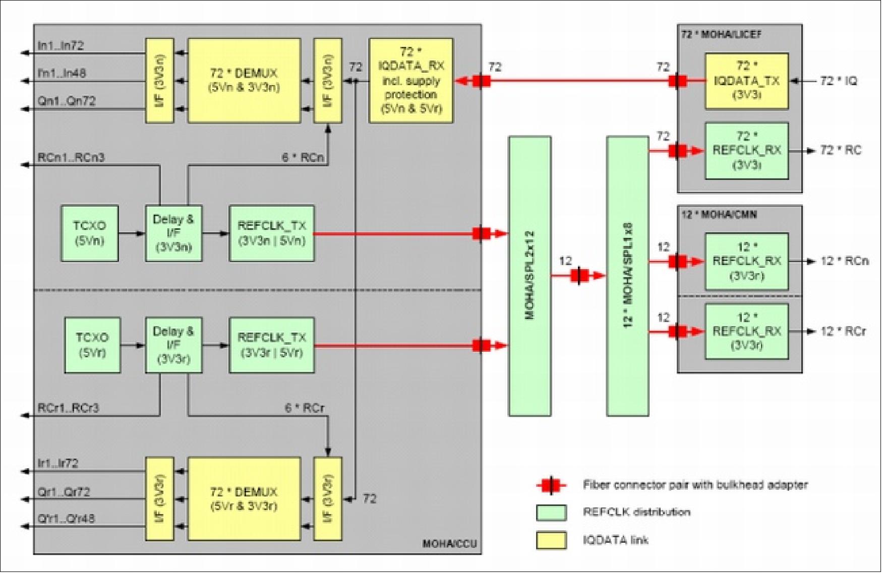
SMOS preparatory and in-flight validation campaigns (technology verification)
• The DOME-Cair (airborne) field campaign was carried out in January 2013 (12-day campaign) at the Concordia research station at Dome-C in Antarctica to validate data from ESA’s SMOS and GOCE missions. The results were presented to ESA in late 2013. This campaign revealed a remarkable similarity between spatial patterns observed by the microwave and gravity instruments (Figure 57). The images also show the flight tracks during the campaign. This could lead to completely new scientific discoveries beneath the surface of the Antarctic ice. 138) 139)
The DOME-Cair campaign was conducted by AWI (Alfred Wegener Institute for Polar and Marine Research) of Bremerhaven, Germany and by DTU [Danmarks Tekniske Universitet (Technical University of Denmark), Lyngby, Denmark].
- The campaign was followed by data quality checks, data processing and the first scientific analyses.
- The aircraft was the AWI Polar-6
- The L-band microwave instrument was the EMIRAD-2 developed by DTU 140)
- The gravimeter (airborne) was the AWI LaCoste-Romberg-Gravimeter.
Based at the isolated Concordia research station at Dome-C, the campaign involved spending two weeks flying a Basler-67 airplane over an area of 350 km2. The plane carried two key sensors: a radiometer used to record surface microwave emissions to verify SMOS data and a gravity meter.
The results of the campaign were presented in late 2013 to ESA and included some major surprises: SMOS and GOCE use completely different types of instruments to measure completely different aspects of Earth. Nevertheless, the measurements taken from the aircraft’s two sensors show similar patterns across the Antarctic ice surveyed by the plane.
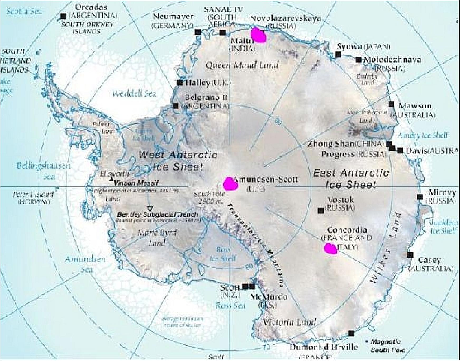
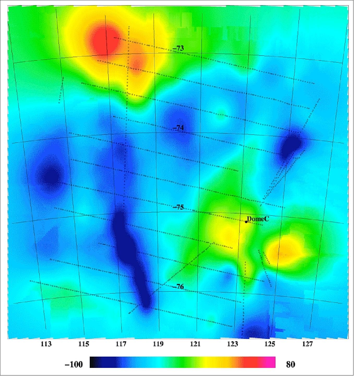
Fully polarimetric (i.e. 4 Stokes) brightness temperatures at the L-band were measured, and are now available on request, along with the final report from DTU (Technical University of Denmark). Figure 58 shows the measured brightness temperature at nadir for vertical (left panel) and horizontal (right panel) polarization over 11 tracks that were acquired over the test area.
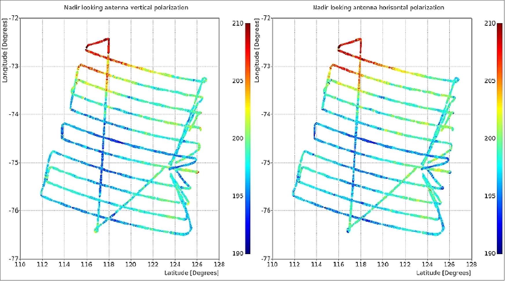
• DOMEX-3 campaign (period: Dec. 2012 to Dec. 2015) at the location DOME-C, Antarctica, providing multi-year, continuous observations of the ice sheet at the Concordia research station in Antarctica. The measurements are made by a new multi-frequency, dual-polarization, passive microwave radiometer positioned on a tower. 141)
This new instrument is based on the Radomex radiometer built by IFAC-CNR’s Institute of Applied Physics in Florence, Italy, which operated successfully in 2008–2010. However, Radomex was not designed for long autonomous operation in the extremely harsh Antarctic climate. The newly designed radiometer will be able to operate autonomously and transmit data to Europe remotely, despite the demanding environment. The radiometer has been calibrated, tested and prepared for shipping to the Concordia station. It is expected to start operations in late 2012, during the austral summer. This multi-year experiment is in support of ESA’s SMOS (Soil Moisture Ocean Salinity) mission.
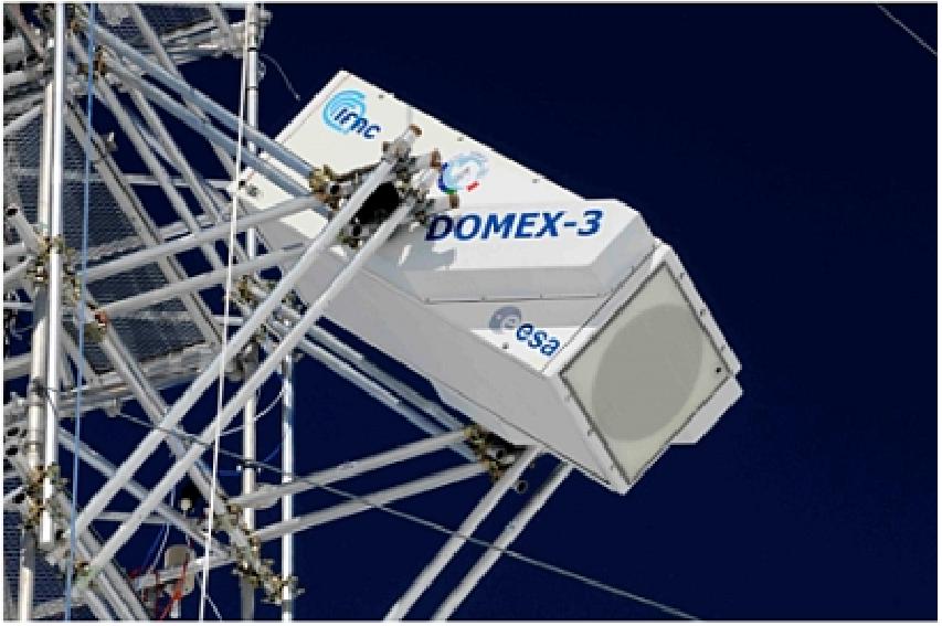
The objectives are:
- Continuous measurement data from the surface of the ice sheet by simultaneous observations from a multi-frequency dual-polarization radiometer and a collocated thermal infrared radiometer over a period of time, spanning multiple annual cycles.
- Collection of time-series brightness temperature measurements at L-band with sufficient calibration accuracy, stability, drift, and of sufficient duration to allow analyses of seasonal variances owing to changes in emission and temperature of the observed snow and ice layers.
- Mitigation and correction for interference sources in the data.
- Provision of external ice-sheet target calibration reference brightness temperature, and the basis for calibration monitoring, and/or verification of brightness temperature products in support of the SMOS mission, especially for re-processing exercises.
- Evaluation of the TEC (Total Electron Content) impact on the temporal stability of the SMOS h-, v-polarised and 1st Stokes parameter measurements in a peak period of Sun activity using Total Electron Content data collected onsite for the duration of the experiment.
DOMEX-3 has so far documented the stability of L-band brightness temperatures over long time periods and hence the suitability of DOME-C for vicarious calibration of L-band radiometers (e.g. SMOS, SMAP and AQUARIUS). 142) 143) 144)
• As ESA's SMOS mission nears the end of its commissioning phase in May 2010, a new ground network, referred to as ISMN (International Soil Moisture Network), will provide harmonized global datasets of soil moisture measurements collected from the ground, ensuring the data received from space are as accurate as possible. 145)
ISMN was set up collaboratively by the following partner institutions: GEWEX (Global Energy and Water Cycle Experiment), GEO (Group on Earth Observations), CEOS (Committee on Earth Observation Satellites), and ESA. ISMN provides an integrative platform to host quality-controlled soil moisture measurements emerging from various ground validation campaigns and operational networks to share freely with the scientific community.
As an important part of the SMOS mission, a number of field campaigns are being carried out to validate the observed data. Both the observed brightness temperature data and the derived data products for soil moisture from SMOS need to be validated.
The soil moisture data from field campaigns can now be fed into ISMN where they are brought into a common volumetric soil moisture unit to allow for accurate comparison with data received from the SMOS spacecraft. This is not as trivial as it may seem because there is neither a standard measurement technique nor a standard protocol for measuring soil moisture. - Hence, the ISMN will advance the process of validation of remotely sensed soil moisture datasets from SMOS and NASA's future SMAP (Soil Moisture Active/Passive) mission, as well as modelled soil moisture data.
Funded by ESA, the Institute of Photogrammetry and Remote Sensing at the Vienna University of Technology (TU Wien, Austria) is responsible for the network (ISMN) and data distribution. ISMN bridges the gap between organizations measuring soil moisture on the ground and people interested in using these data. - For improved worldwide validation of satellite and model estimates of soil moisture, all campaign and operational soil moisture networks are welcome to share their data with the scientific community through the ISMN (International Soil Moisture Network).
ESA's SMOS campaigns: Three preparatory campaigns were conducted during the Phase-A study period to analyze signal dependence and validate existing and improved models. The campaigns were: 146) 147) 148)
• WISE (Wind and Salinity Experiment). WISE was conducted in 2000 (Nov. 25 to Dec. 18, 2000) and 2001 (Jan. 9 to 16, 2001) from an oil rig, about 50 km off the coast of Tarragona in the northwest Mediterranean. The experiments were conducted by UPC (Technical University of Catalonia), and ICM (Institute of Marine Sciences) both of Barcelona, Spain. The LAURA (UPC L-band AUtomatic RAdiometer) was deployed in REPSOL's Casablanca oil rig, in conjunction with other oceanographic and meteorological instrumentation. Study of the impact on the brightness temperature of sea state, as well as the effect of wave development, swell, currents, rain, and oil spills; retrieval of sea surface salinity from multi-angular polarimetric L-band radiometric data. 149) 150) 151) 152)
• EuroSTARRS (Salinity Temperature and Roughness Remote Scanner in Europe). The objective of EuroSTARRS-2001 was to acquire SMOS-like observations for addressing the critical issues relevant to the soil-moisture objectives of the SMOS mission. STARRS, owned by NRL (Washington, DC), was operated during the campaign aboard a Dornier-228 by DLR, Oberpfaffenhofen.
• LOSAC (L-band Ocean Salinity Campaign). The objective of LOSAC was to address azimuthal dependence of the first two Stokes parameters (Tb,v and Tb,h) on wind speed and direction. The EMIRAD polarimetric L-band radiometer of TUD (Technical University of Denmark) was used aboard the C130 aircraft operated by the Royal Dutch Air Force over the North Sea. First flights were conducted in 2001. Overall, the campaign lasted until 2003. 153)
• DOMEX (Microwave Emission of the East Antarctica Plateau): An experimental campaign (DOMEX) with ground based radiometers was carried out at Dome-C in the summer 2004/2005 to control the stability of L- and C -band emission at a monthly scale, within the framework of the ESA-SMOS calibration and validation activities. The DOMEX campaign was organized with CNR-IFAC, Florence, Italy. The campaign (tower-based measurements) took place in Dec. 2004 at DOME-CONCORDIA in Antarctica. The campaign concluded in 2005.
• CoSMOS-2, Airborne measurements in Australia in Nov. 2005 (Aero Commander aircraft of Flinders University, Adelaide), dedicated to SM (Soil Moisture) observations. Cooperation with the Australian University of Melbourne, Newcastle in the framework of the National Australian Field Experiment (NAFE). Participation of European Teams [Free University of Amsterdam, (The Netherlands), University of Valencia (Spain), CESBIO (France)]. The objective of the CoSMOS airborne campaign was to perform a “long-term” acquisition of data under different geo/bio-physical as well as meteorological and oceanographic conditions to address open issues related to the retrieval and validation of the SMOS products.
• CoSMOS-OS with the goal to map sea surface salinity: An airborne campaign (4 weeks) in Norway in April 2006 using the second generation EMIRAD (Electromagnetics Institute Radiometer) digital detection instrument of TUD (Technical University of Denmark) on the Skyvan aircraft of HUT/TKK (Helsinki University of Technology), Finland. The objective was to perform the acquisition of data under different oceanographic conditions to address open issues related to the retrieval and validation of the SMOS products. For all flights, the time at the target has been chosen to coincide with an ENVISAT/ASAR overpass to obtain information about the actual surface roughness, and meteorological information was provided from oil-drilling installations in the target area. 154) 155)
• SAM (Small-scale Airborne prototype of MIRAS). ESA-CASA is developing SAM as prime contractor within the framework of the MDPP-3 project (MIRAS Demonstrator Pilot Project-3), sponsored by ESA. Several European institutions are participating in the development of the MDPP-3 instrument and test campaigns (UPC, HUT, etc.). The SAM demonstrator consists of 12 LICEF receivers (4 per arm), 1 reference radiometer (NIR) and includes the same internal calibration system scheme as foreseen for MIRAS. 156)
In the near future, SAM will be flown in a light aircraft, the Skyvan of the LST/HUT (Laboratory of Space Technology/Helsinki University of Technology), to undertake several airborne campaigns over land and sea. These airborne campaigns are devised to test the capability of SMOS calibration and retrieval algorithms to provide soil moisture and ocean salinity in the natural environment.
• TuRTLE (Topography effects on RadiomeTry at L-band Experiment). UPC (Spain) carried out a set of experiments to study the impact of different soil and vegetation properties on land emission: 157)
- The vine canopy, observation position, and soil moisture (SMOS REFerence pixel L-band Experiment, REFLEX, 2003 and 2006
- The soil type, and moisture profile (MOnitoring Underground Soil Experiment, MOUSE, 2004, and the soil roughness (Terrain-Roughness EXperiments T-REX, 2004 and 2006
The objective of TuRTLE was to acquire radiometric measurements of pixels with changing topography and to compare them to existing brightness temperature models. TuRTLE 2006 was carried out in a mountainous area about 50 km North of Barcelona (Spain). Radiometric measurements covering the mountain slope, and up to the sky were acquired. Concurrently, ground truth and meteorological data were registered. Radiometric measurements have been compared to the emissivity obtained by simulation using a facet model which considers the high-resolution digital elevation model and land cover map of the area. Polarization mixing due to surface tilting and integration over the antenna pattern has also been included in the simulator, and the results agree with the radiometric measurements.
The campaign was carried out in May 12-19, 2006. The radiometric data was acquired by the UPC full-polarimetric, Dicke radiometer LAURA (L-band AUtomatic RAdiometer. The mountainous scene in front of the radiometer was observed at seven elevation (from 45º-to 105º referred to nadir, in 10º steps) and nine azimuth angles, covering the mountain slope terrain and the mountain-sky transition.
• AMIRAS (Airborne MIRAS) is a new instrument that is similar to the MIRAS radiometer on SMOS. AMIRAS, however, is much smaller than MIRAS and designed to operate from an aircraft to provide scientists with data similar to those expected from the SMOS mission. In Dec. 2006, AMIRAS has successfully delivered images from its maiden flight over Finland. AMIRAS consists of a Y-shaped array with four antennae elements per arm. It had its maiden flight onboard the Helsinki University of Technology's (HUT, also referred to as TKK) Skyvan in June 2006 covering both land and sea areas around Helsinki, Finland. EADS-CASA Espacio, Spain, is the prime contractor for AMIRAS. The AMIRAS instrument consists of 12 receivers (4 per arm), and 1 reference radiometer (NIR) and includes the internal calibration system foreseen for MIRAS. 158) 159)
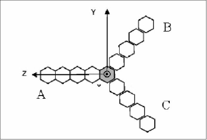
• HUT-2D (Helsinki University of Technology 2D Radiometer). HUT-2D is an airborne L-band two-dimensional interferometric radiometer using aperture synthesis. The instrument was designed and manufactured at LST (Laboratory of Space Technology) of HUT (Helsinki University of Technology) in cooperation with Ylinen Electronics Ltd., Finland. The HUT-2D radiometer instrument consists of 36 receivers, a local oscillator subsystem, a calibration subsystem and a one-bit digital correlator unit. Each pair of receivers (baseline) builds a correlating receiver. The cross-correlation of the receiver outputs are processed in the correlator unit. The radiometer has been accommodated below the fuselage of the HUT remote sensing aircraft (Short SC-7 Skyvan) using three specifically designed attachment points.
In 2006 and 2007, the HUT-2D instrument represented a significant contribution to the SMOS mission preparatory campaigns in providing the first successful airborne demonstration of the complete system. This complex and sophisticated instrument has been used in calibration and validation campaigns to assess retrieval algorithms for soil moisture and ocean salinity. The instrument, even though the antennas are in a different configuration (U-shape vs Y-shape on MIRAS), is very suitable for various verification and validation methods for the MIRAS instrument of SMOS. 160)
• AACES (Australian Airborne Calibration/Validation Experiments for SMOS). The AACES campaign was underway between mid-January and the end of February 2010 in the Murrumbidgee catchment in southern New South Wales, Australia. Given the recent launch of SMOS (Nov. 2, 2009), AACES represents the first extensive and probably most comprehensive of such experiments undertaken during the commissioning and later operational phase of SMOS. The project was led by Jeff Walker and Chris Rudiger from the University of Melbourne and supported by the invaluable help of their PhD students. Moreover, thanks to the generosity of various research institutes from France, Germany, Denmark, Poland, and the Netherlands in addition to the flights covered by ESA, a total of 14 people have joined this campaign to boost the manpower of the sampling teams. 161) 162) 163)
The Murrumbidgee catchment is unique as it comprises a distinct variety of topographic, climatic and land cover characteristics, and therefore represents an excellent validation site for the land component of this satellite mission. A total of 10 patches of 100 km x 50 km (aligned with the synthetic SMOS grid, and therefore including two independent SMOS footprints) are covered by an aircraft carrying an L-band radiometer and VIS/NIR/SWIR/TIR sensors. 164)
With a flight altitude, the ground pixel resolution is 1km, resulting in almost complete coverage of the catchment transect of 500 km. The aircraft flights are aligned with SMOS morning overpasses. At the same time, two ground teams are covering an area of 5km x 2km each, collecting soil moisture (50 m spacing along the 5 km transects), soil temperature, and soil salinity. A sub-group of each team was in parallel collecting LAI, dew, destructive vegetation samples, and hyperspectral measurements of the surface conditions.
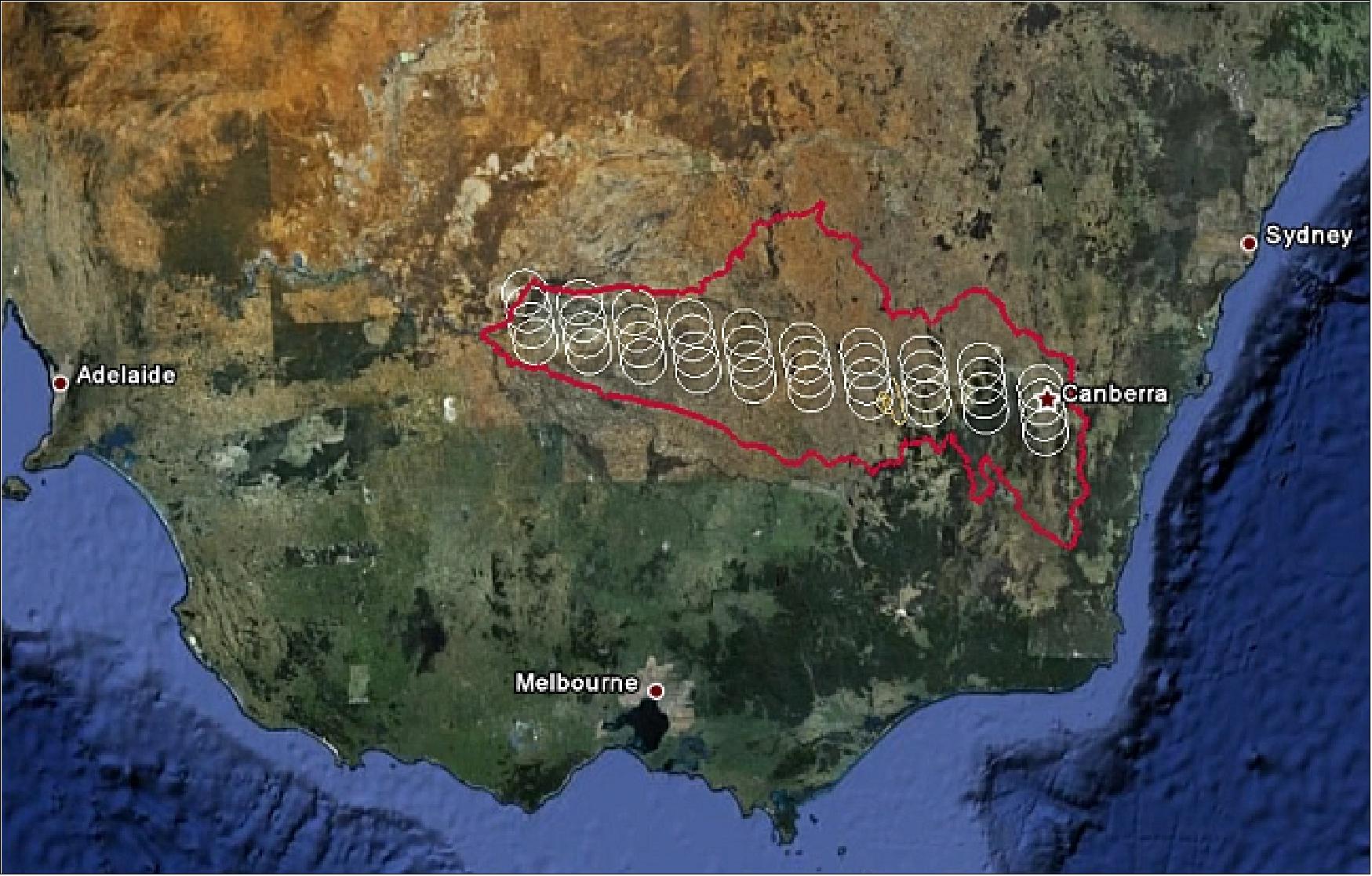
SMOS Ground Segment
SMOS is an ESA Earth Explorer mission with significant national contributions provided by the French and Spanish space agencies, CNES and CDTI. The collaborative approach for the development of the SMOS mission will be continued in the operations phase, with the ground segment consisting of different stations covering various functions. For the operations phase, ESA will be responsible for the overall coordination of the mission and the ground segment operations, and CNES will be operating the spacecraft. 165)
The main stations for day-to-day running will be ESA’s European Space Astronomy Centre (ESAC), in Spain, hosting the main part of the Data Processing Ground Segment (DPGS), and CNES at Toulouse, hosting the Satellite Operations Ground Segment (SOGS). Global soil moisture data are important variables for operational meteorological applications.
The SMOS ground segment is composed of the following components: 166) 167) 168) 169)
1) SOGS (Satellite Operations Ground Segment) located at CNES in Toulouse, France.
2) DPGS (Data Processing Ground Segment) of ESA/CDTI (ESA/Centro para el Desarrollo Technologico Industrial), located at ESA/ESAC (European Space Astronomy Centre) in Villafranca, Spain - and at ESA/ESRIN (user interface) in Frascati, Italy. DGPS is devoted to acquire, process, and dispatch the SMOS data product levels L1 and L2 (L1A, L1B, L1Csm, L1Cos, L2Csm, L2Cos) to the user community (Figure 64).
The following elements provide the main functions for DPGS: 170) 171)
- SPGF (SMOS Plan Generation Facility): Instrument and acquisition planning information
- Data are acquired with the 3.5 m XBAS (X-Band Acquisition System) receiving antenna
- PXMF (Payload X-Band Monitoring Facility) is part of PLPC development. It provides a means for the operator to monitor the X-band telemetry
- CEC (Calibration Engineering Centre). CEC provides product quality [SPQC (SMOS Product Quality Control)], calibration and validation tools, and system-level monitoring.
3) CATDS (Centre Aval de Traitement des Donnees SMOS) is at CNES, dedicated to process, archive, and dispatch the SMOS data product levels L3 and L4 (Figure 65). The product levels L3 and L4 are derived from the L1 and L2 levels. Note: IFREMER will be in charge of CATDS operations to optimize costs and the maximum reuse of data. 172)
4) PLPC (Payload Operations and Programming Centre) at ESA/ESAC, Villafranca, Spain.
In 2006, ESA member states approved an add-on to the original mission configuration by introducing another X-band receiving station at Svalbard, Norway, which will guarantee this service. Above the Arctic Circle, Svalbard will provide 10 out of the 14 orbits per day that ESAC is not able to acquire in real-time due to its geographical location (Ref. 165).
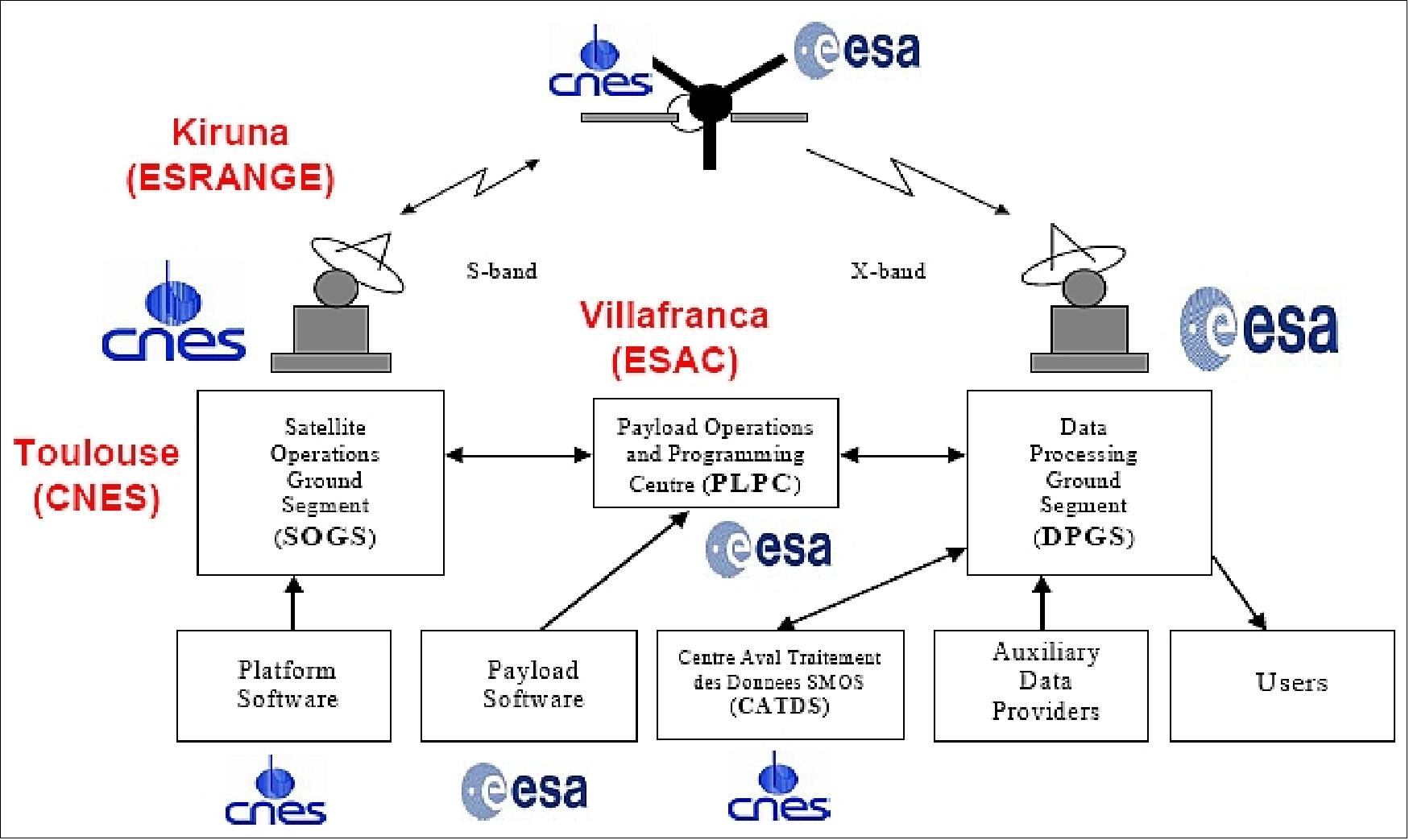
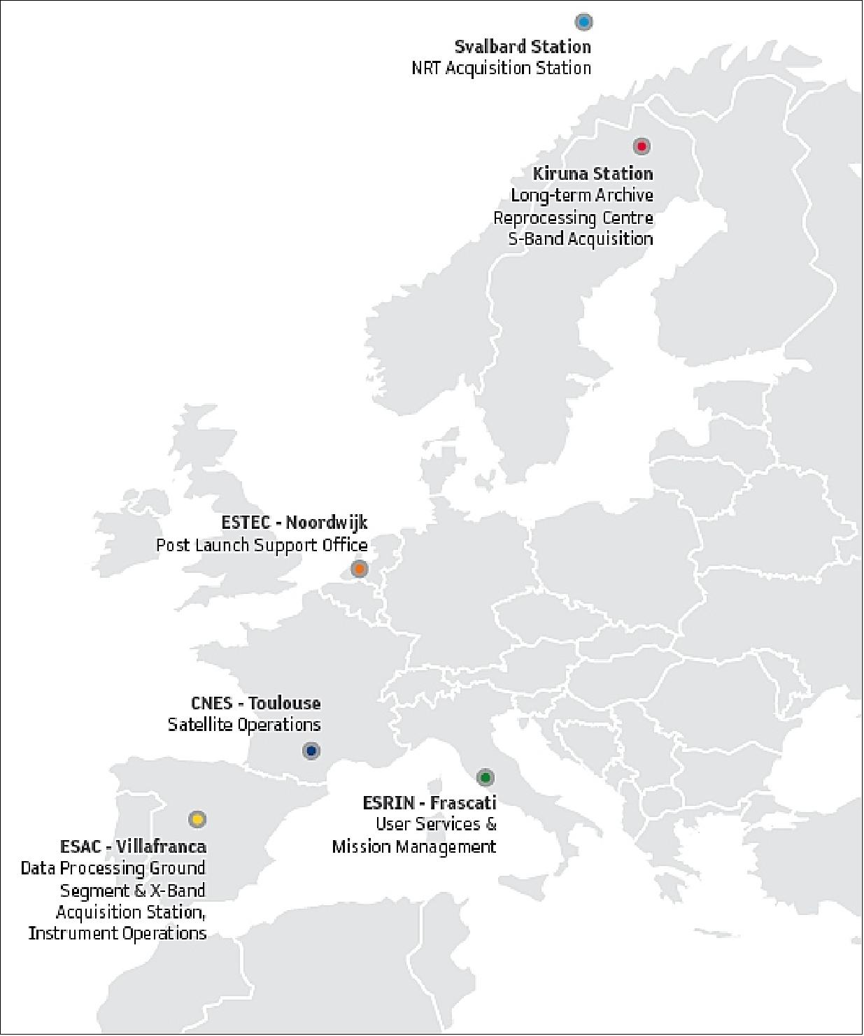
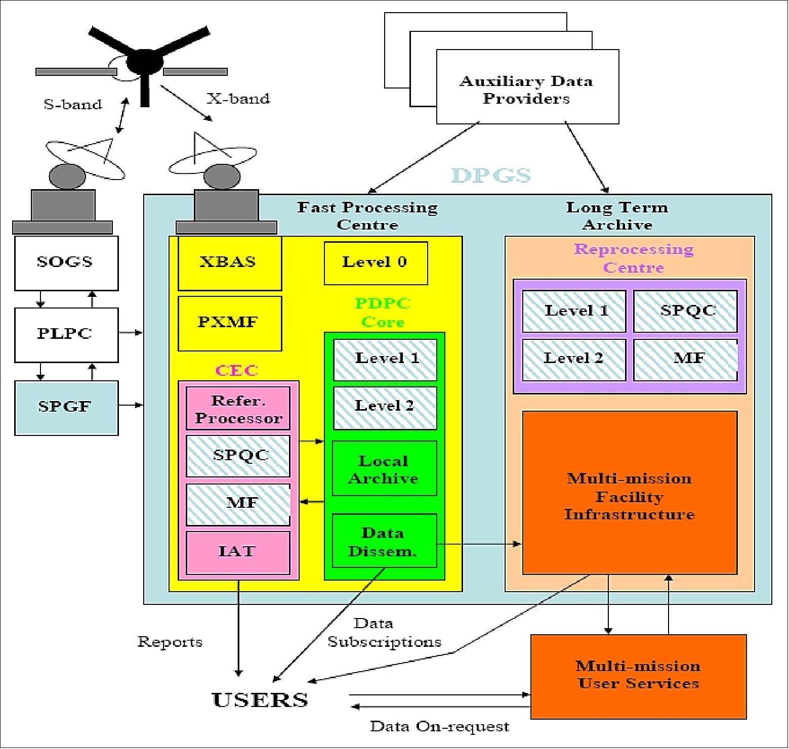
In addition, further data services will be provided:
• IFREMER [Institut Francais de Recherche pour L'Exploration de la Mer (French Ocean Agency in Brest, France)] will provide the oceanographic community with a homogeneous time series of value-added data relevant to the sea surface state (wind fields, fluxes, waves or sea-ice)
• CESBIO [Centre d'Études Spatiales de la Biosphére (Toulouse, France)] will host the SM Expertise Centre; and will deliver the L3+L4 algorithms specifications and mock-up (with the help of the other laboratories involved in L3/L4 SM)
• IFREMER will host the OS Expertise Centre; and will deliver the L3+L4 algorithms specifications and mock-up (with the help of the other laboratories involved in L3/L4 OS)
• ECMWF [European Centre for Medium-Range Weather Forecasts (Reading, UK)] will provide key auxiliary data of ocean and land
• Spain (CDTI, UPC, INDRA Espacio). Spain will develop CP34, another ground-segment dedicated to SMOS L3+L4 products processing
• etc.
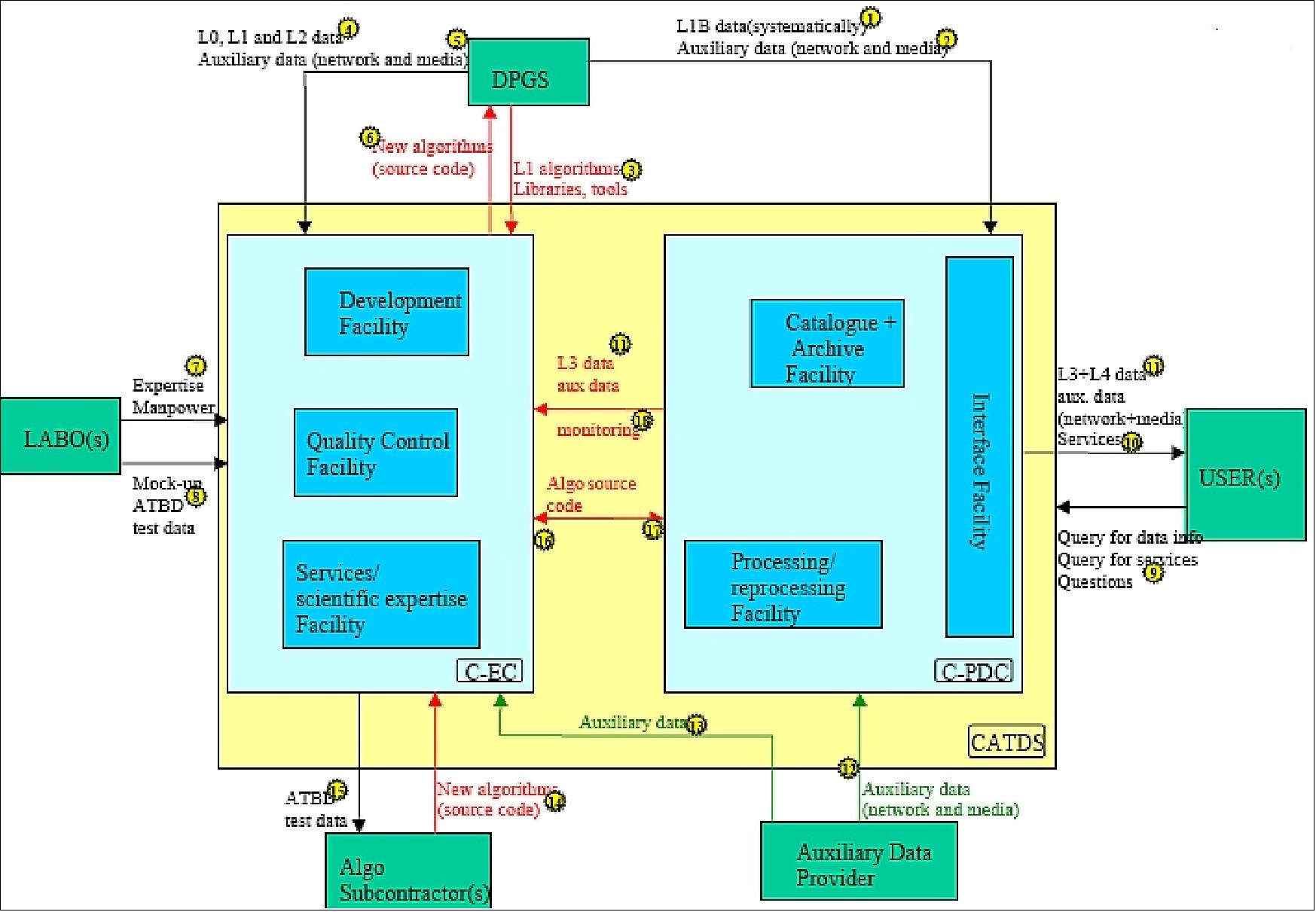
SMOS data product level objectives:
- L1/L2: The SMOS SM (Soil Moisture) objective is accuracy of 4% on volumetric soil moisture, with three days revisit and a sampling step better than 50 km.
- L1/L2: The SMOS OS (Ocean Salinity) objective is an accuracy better than 0.1 PSU, with 10 days to monthly grid scale (200 km). Knowing that a single measurement will be poor (~1 PSU), spatial and temporal averages will be needed to reduce the noise.
- L3: L3SM will consist of soil moisture global maps (regular grid 0.15º x 0.15º), produced every day and based on the three previous days.
- L3 OS maps are produced every day with GODAE (Global Ocean Data Assimilation Experiment) specifications (5-10 days sliding maps with a 200 km x 200 km resolution).
References
1) M. Martin-Neira and the SMOS Project Team, “The Soil Moisture and Ocean Salinity (SMOS) Mission,” URSI 2005 Commission F Symposium on Microwave Remote Sensing of the Earth, Oceans, Ice, and Atmosphere, Ispra, Italy, April 20-21, 2005
2) P. Silvestrin, M. Berger, Y. H. Kerr, J. Font, ”ESA's Second Earth Explorer Opportunity Mission: The soil Moisture and Ocean salinity Mission - SMOS.” IEEE Geoscience and Remote Sensing Newsletter (118), 2001, pp.11-14
3) J. Blouvac, B. Lazaed, J. M. Martinuzzi, “ CNES Small Satellites Earth Observation Scientific Future Missions, IAA 2nd International Symposium on Small Satellites for Earth Observation, Berlin, April 12-16, 1999, pp. 11-14
4) Y. H. Kerr, P. Waldteufel, J.-P. Wigneron, J. Font, M. Berger, “The Soil Moisture And Ocean Salinity Mission,” Proceedings of IEEE/IGARSS 2003, Toulouse, France, July 21-25, 2003
5) H. M. J. P. Barre, B. Duesmann, Y. H. Kerr, “SMOS: The Mission and the System,” IEEE Transactions on Geoscience and Remote Sensing, Vol. 46, No 3, March 2008, pp. 587-593
6) Mark Drinkwater, Yann Kerr, Jodi Font, Michael Berger, “Exploring the Water Cycle of the 'Blue Planet',” ESA Bulletin, No 137, Feb. 2009, pp. 6-15
7) M. Martin-Neira, J. Font, M. Srokosz, I. Corbella, A. Camps, “Ocean Salinity Observations with SMOS Mission,” Proceedings of the IEEE IGARSS 2000 Conference, Honolulu, HI, July 24-28, 2000
8) Y. H. Kerr, P. Waldteufel, J.-P. Wigneron, J. Font, “The Soil Moisture and Ocean Salinity Mission: The Science Objectives of an L-band 2-D Interferometer,” Proceedings of the IEEE IGARSS 2000 Conference, Honolulu, HI, July 24-28, 2000
9) Y. Kerr, J. Font, et al., “Next Generation Radiometers: SMOS - A Dual Pol L-band 2-D Apertures Synthesis Radiometers,” 2000 IEEE Aerospace Conference, March 2000, Montana,USA
10) Y. H. Kerr, J. Font, P. Waldteufel, M. Berger, “The Soil Moisture and Ocean Salinity Mission -SMOS,” ESA Earth Observation Quarterly, No 66, July 2000, pp. 18-26
11) Y. H. Kerr, P. Waldteufel, J. P. Wigneron, J. Font, “Description of the Soil Moisture and Ocean Salinity Mission,” COST 712 -WG 3 report, 2001, European Union, Brussels
12) http://www.cesbio.ups-tlse.fr/us/indexsmos.html
13) M. Berger, A. Camps, J. Font, Y. Kerr, et al., “Measuring Ocean Salinity with ESA's SMOS Mission,” ESA Bulletin 111, Aug. 2002, pp. 113-121
14) F. Bermudo, M. Venet, M. Le du, Y. Kerr , H. Barre, “SMOS: An L-band Interferometric Radiometer Mission,” 5th IAA Symposium on Small Satellites for Earth Observation, April 4-8, 2005, Berlin, Germany
15) http://www.esa.int/esaLP/ESAL3B2VMOC_LPsmos_0.html
16) J. P. Wigneron, A. Chanzy, P. Waldteufel, J. C. Calvet, O. Marloie, J. P. Hanocq, Y. H. Kerr, “Retrieval capabilities of L-Band 2-D interferometric radiometry over land surfaces (SMOS Mission), VSP, Netherlands, 2000
17) J. P. Wigneron, P. Waldteufel, A. Chanzy, J. C. Calvet, Y. H. Kerr, ”Two-D microwave interferometer retrieval capabilities of over land surfaces (SMOS Mission),” Remote Sensing Environment, Vol. 73, No 3, 2000, pp. 270-282
18) “SMOS: ESA's Water Mission,” BR-224, June 2004, brochure of 20 pages, URL: http://esamultimedia.esa.int/docs/br_224.pdf
19) M. Berger, Y. Kerr, J. Font, J.-P. Wigneron, et al., “Measuring the Moisture in the Earth's Soil - Advancing the Science with ESA's SMOS Mission,” ESA Bulletin No 115, Aug. 2003, pp. 40-45, URL: http://www.esa.int/esapub/bulletin/bullet115/chapter5_bul115.pdf
20) Y. Kerr, P. Waldteufel, F. Cabot, A. Hahne, S. Mecklenburg, Thierry Pellarin, “The SMOS Mission Current Status,” Earth Observation and Water Cycle Science - Towards a Water Cycle Multi-mission Observation Strategy, ESA/ESRIN, Frascati, Italy, Nov. 18-20, 2009
21) M. Martin-Neira, “MIRAS - A Two-Dimensional Aperture-Synthesis Radiometer for Soil-Moisture and Ocean-Salinity Observations,” ESA Bulletin No 92, Nov. 1997, URL: http://www.esa.int/esapub/bulletin/bullet92/b92marti.htm
22) Francois Bermudo, Michel Venet, Michel Ledu, Yann Kerr, “SMOS - An L-band Interferometric Radiometer Mission,” Proceedings of the 60th IAC (International Astronautical Congress), Daejeon, Korea, Oct. 12-16, 2009, IAC-09-B1.1.2
23) Michel Le Du, Roger Jegou, “SMOS Mission, a Successful Cooperation based on the Flight Proven PROTEUS Platform,” Proceedings of the Symposium on Small Satellite Systems and Services (4S), Funchal, Madeira, Portugal, May 31-June 4, 2010
24) Mariano Kornberg, Elena Checa, Silvio Dolce, Manuel Martin-Neira, Pilar Rubiales, Josep Closa, Guillermo Buenadicha, Jorge Fauste, “Thermal Control in SMOS Payload Operations: Anomalies, Seasonal Effects, Failure & Recovery Issues,” SpaceOps 2014, 13th International Conference on Space Operations, Pasadena, CA, USA, May 5-9, 2014
25) “Two new ESA satellites successfully lofted into orbit,” ESA, Nov. 2, 2009, URL: http://www.esa.int/esaCP/SEMNEYAOE1G_index_0.html
26) “Final look at ESA’s SMOS and Proba-2 satellites,” ESA, Oct. 21, 2009, URL: http://www.esa.int/esaCP/SEMMX8ZRA0G_index_0.html
27) http://earth.esa.int/SMOS/
28) Note: The revisit cycle is the frequency at which any point on the globe is seen again at any position within the swath. The repeat cycle is the frequency at which any point on the globe is seen again at the same position within the swath.
29) ”Forest degradation primary driver of carbon loss in the Brazilian Amazon,” ESA / Applications / Observing the Earth / Space for our climate, 10 June 2021, URL: https://www.esa.int/Applications/Observing_the_Earth/Space_for_our_climate
/Forest_degradation_primary_driver_of_carbon_loss_in_the_Brazilian_Amazon
30) Yuanwei Qin, Xiangming Xiao, Jean-Pierre Wigneron, Philippe Ciais, Martin Brandt, Lei Fan, Xiaojun Li, Sean Crowell, Xiaocui Wu, Russell Doughty, Yao Zhang, Fang Liu, Stephen Sitch & Berrien Moore III, ”Carbon loss from forest degradation exceeds that from deforestation in the Brazilian Amazon,” Nature Climate Change, Vol. 11, pp: 442-448, Published: 29 April 2021, https://doi.org/10.1038/s41558-021-01026-5
31) ”The ripple effect: Solving source of irregularities in images sent back by SMOS,” ESA Enabling & Support, 05 May 2021, URL: https://www.esa.int/Enabling_Support/Space_Engineering_Technology
/The_ripple_effect_Solving_source_of_irregularities_in_images_sent_back_by_SMOS
32) ”Water mission takes on space weather,” ESA Applications, 24 March 2021, URL: http://www.esa.int/Applications/Observing_the_Earth/SMOS/Water_mission_takes_on_space_weather
33) M. Flores‐Soriano, C. Cid, R. Crapolicchio, ”Validation of the SMOS mission for Space Weather operations: The potential of near real‐time solar observation at 1.4 GHz,” AGU Space Weather, Published: 08 February 2021, https://doi.org/10.1029/2020SW002649
34) ”SMOS monitoring droughts,” ESA Applications, 23 June 2020, URL: http://www.esa.int/ESA_Multimedia/Videos/2020/06/SMOS_monitoring_droughts
35) ”Czech Republic drought visible from space,” ESA / Applications / Observing the Earth / SMOS, 18 May 2020, URL: http://www.esa.int/Applications/Observing_the_Earth
/SMOS/Czech_Republic_drought_visible_from_space
36) ”New maps of salinity reveal the impact of climate variability on oceans,” ESA / Applications / Observing the Earth / Space for our climate, 30 November 2019, URL: http://www.esa.int/Applications/Observing_the_Earth/Space_for_our_climate/
New_maps_of_salinity_reveal_the_impact_of_climate_variability_on_oceans
37) ”Space is key to monitoring ocean acidification,” ESA / Applications / Observing the Earth / SMOS, 28 November 2019, URL: http://www.esa.int/Applications/Observing_the_Earth
/SMOS/Space_is_key_to_monitoring_ocean_acidification
38) ”Revealing interior temperature of Antarctic ice sheet,” ESA / Applications / Observing the Earth / SMOS, 04 November 2019, URL: http://www.esa.int/Applications/Observing_the_Earth
/SMOS/Revealing_interior_temperature_of_Antarctic_ice_sheet
39) Giovanni Macelloni, Marion Leduc-Leballeur, Francesco Montomoli, Marco Brogioni, Catherine Ritz, Ghislain Picard, ”On the retrieval of internal temperature of Antarctica Ice Sheet by using SMOS observations,” Remote Sensing of Environment, Volume 233, November 2019, 111405, https://doi.org/10.1016/j.rse.2019.111405
40) ”SMOS 10 years in orbit,” ESA, 31 October 2019, URL: http://www.esa.int/ESA_Multimedia/Videos/2019/10/SMOS_10_years_in_orbit
41) E. Uranga, A. Llorente, A. de la Fuente, E. Daganzo, R. Oliva and Y. Kerr, ”Radio frequency interference devices: The SMOS experience,” Proceedings of the 39th annual IGARSS (International Geoscience and Remote Sensing Symposium) 2019, Yokohama, Japan, 28 July - 2August 2019
42) E. Uranga, A. Llorente, R. Oliva, A. de la Fuente, E. Daganzo and Y. Kerr, "Monitoring of Smos Rfi Sources in the 1400-1427mhz Passive Band," IGARSS 2018 - 2018, IEEE International Geoscience and Remote Sensing Symposium, Valencia, 2018, pp. 1241-1244
43) R. Oliva, E. Daganzo, P. Richaume, Y. Kerr, F. Cabot, Y. Soldo, E. Anterrieu, N. Reul, A. Gutierrez, J. Barbosa, and G. Lopes, “Status of Radio Frequency Interference (RFI) in the 1400–1427MHz passive band based on six years of SMOS mission”, Remote Sensing of Environment, Vol. 180, July 2016, pp. 64-75
44) E. Uranga, Á. Llorente and A. de la Fuente, “Database of SMOS RFI sources in the 1400-1427MHz passive”, IEEE Global Conference on Signal and Information Processing, Anaheim, California, USA, November 2018.
45) ”SMOS joins forces with top weather forecasting system,” ESA, 12 June 2019, URL: http://www.esa.int/Our_Activities/Observing_the_Earth
/SMOS/SMOS_joins_forces_with_top_weather_forecasting_system
46) ”Mapping salty waters,” ESA, Space for our climate, 14 May 2019, URL: http://www.esa.int/Our_Activities/Observing_the_Earth
/Space_for_our_climate/Mapping_salty_waters
47) ”New potential for tracking severe storms,” ESA Observing the Earth, 14 May 2019, URL: http://www.esa.int/Our_Activities/Observing_the_Earth
/SMOS/New_potential_for_tracking_severe_storms
48) ”SMOS severe winds over ocean – first operational data products tested,” SMOS Newsletter, Issue 16, November 2018, URL: https://earth.esa.int/
documents/10174/234899/SMOS-Newsletter-16-November-2018
49) ”SMOS offers new perspective on hurricanes,” ESA, 25 September 2018, URL: http://m.esa.int/Our_Activities/Observing_the_Earth/
SMOS/SMOS_offers_new_perspective_on_hurricanes
50) ”SMOS simplified data access,” ESA, 23 August 2018, URL: [web source no longer available]
51) Manuel Martín-Neira, Roger Oliva, Ignasi Corbella, Francesc Torres, Nuria Duffo, Israel Durán, Juha Kainulainen, Josep Closa, Alberto Zurita, François Cabot, Ali Khazaal, Eric Anterrieu, Jose Barbosa, Gonçalo Lopes, Joe Tenerelli, Raúl Díez-García, Jorge Fauste, Antonio Turiel, Verónica González-Gambau, Raffaele Crapolicchio, Martin Suess,”SMOS instrument performance after more than 8 years in orbit and lessons learned for future L-band missions,” Proceedings of IGARSS (International Geoscience and Remote Sensing Symposium), Valencia, Spain, July 23-27, 2018
52) ”SMOS Newsletter — 'Data an Processors' p. 3,” 15 July 2018, URL: https://earth.esa.int/documents/10174/234899/SMOS-Newsletter-15-July-2018
53) ”Six years of the new SMOS SSS maps in the Mediterranean Sea now available!,” BEC (Barcelona Expert Center), 6 April 2018, URL: http://bec.icm.csic.es/
six-years-of-the-new-smos-sss-maps-in-the-mediterranean-sea-now-available/
54) Estrella Olmedo, Isabelle Taupier-Letage, Antonio Turiel, Aida Alvera-Azcárate, ”Improving SMOS Sea Surface Salinity in the Western Mediterranean Sea through Multivariate and Multifractal Analysis,” Remote Sensing, 2018, 10(3), 485; doi:10.3390/rs10030485, URL: http://www.mdpi.com/2072-4292/10/3/485/pdf
55) ”Programs in Progress: SMOS,” ESA Bulletin No 170, 22 September 2017, p.52, URL: http://www.esa.int/About_Us/ESA_Publications/ESA_Publications_Bulletin/ESA_Bulletin_170_2nd_quarter
56) ”Italy’s drought seen from space,” ESA, 5 Sept. 2017, URL: http://m.esa.int/Our_Activities/Observing_the_Earth/Italy_s_drought_seen_from_space
57) Manuel Martín-Neira, Roger Oliva, Ignasi Corbella, Francesc Torres, Nuria Duffo, Israel Durán, Juha Kainulainen, Josep Closa, Alberto Zurita, François Cabot, Ali Khazaal, Eric Anterrieu, José Barbosa, Gonçalo Lopes, Joe Tenerelli, Raúl Díez-García, Jorge Fauste, Verónica González-Gambau, Antonio Turiel, Steven Delwart, Raffaele Crapolicchio, Martin Suess, Susanne Mecklenburg, Matthias Drusch, Roberto Sabia, Elena Daganzo-Eusebio, Yann Kerr, Nicolas Reul, ”Lessens learnt from SMOS after 7 years in orbit,” Proceedings of IGARSS 2017 (IEEE International Geoscience and Remote Sensing Symposium), Fort Worth, Texas, USA, July 23–28, 2017
58) ”Satellites forewarn of locust plagues,” ESA, June 13, 2017, URL: http://m.esa.int/Our_Activities/Observing_the_Earth/Satellites_forewarn_of_locust_plagues
59) ”SMOS brings Mediterranean salinity into focus,” ESA, 11 May 2017, URL: http://m.esa.int/Our_Activities/Observing_the_Earth/
SMOS/SMOS_brings_Mediterranean_salinity_into_focus
60) ”Satellite cousins have ice covered,” ESA, Dec. 16, 2016, URL: http://m.esa.int/Our_Activities/Observing_the_Earth/SMOS/Satellite_cousins_have_ice_covered
61) ”SMOS on speed,” ESA, Oct. 14, 2016: URL: http://m.esa.int/Our_Activities/Observing_the_Earth/SMOS/SMOS_on_speed
62) ”Soil moisture processed two ways,” ESA, Oct. 14, 2016, URL: http://m.esa.int/spaceinimages/Images/2016/10/Soil_moisture_processed_two_ways
63) ”Wet soils following extensive rainfall,” ESA, Oct. 14, 2016, URL: http://m.esa.int/spaceinimages/Images/2016/10/Wet_soils_following_extensive_rainfall
64) ”Zooming in on moisture,” ESA, Oct. 14, 2016, URL: http://m.esa.int/spaceinimages/Images/2016/10/Zooming_in_on_moisture
65) Manuel Martín-Neira, Roger Oliva, Ignasi Corbella, Francesc Torres, Núria Duffo, Israel Durán, Juha Kainulainen, Josep Closa, Alberto Zurita, François Cabot, Ali Khazaal, Eric Anterrieu, Jose Barbosa, Gonçalo Lopes, Joe Tenerelli, Raúl Díez-García, Jorge Fauste, Verónica González-Gambau, Antonio Turiel, Steven Delwart, Raffaele Crapolicchio, Martin Suess, ”SMOS instrument performance and calibration after 6 years in orbit,” Proceedings of the IEEE IGARSS (International Geoscience and Remote Sensing Symposium) Conference, Beijing, China, July 10-15, 2016
66) Michael Rast, ”ESA’s Report to the 41st COSPAR Meeting,”(ESA SP-1333, June 2016), Istanbul, Turkey, July-August 2016, ”Soil Moisture and Ocean Salinity (SMOS),” pp: 28-32, URL: http://esamultimedia.esa.int/multimedia/publications/SP-1333/SP-1333.pdf
67) J. Boutin, N. Martin, G. Reverdin ,J. L. Vergely, ”Rainfall Imprint on SMOS Sea Surface Salinity,” Earth Observation for Water Cycle Science 2015, Frascati, Italy, 20-23 October, 2015, URL: http://www.eo4water2015.info/
68) Yann Kerr, ”SMOS The Water Cycle Mission: An Overview,” Earth Observation for Water Cycle Science 2015, Frascati, Italy, 20-23 October, 2015, URL: http://www.eo4water2015.info/
69) ”SMOS meets ocean monsters,” ESA, Sept. 30, 2015, URL: http://www.esa.int/Our_Activities/Observing_the_Earth/SMOS/SMOS_meets_ocean_monsters
70) S. Mecklenburg, M. Drusch, Y. Kerr, J. Font, N. Reul, M. Martin-Neira, S. Delwart, R. Crapolicchio, J. Fauste, E. Daganzo-Eusebio, A. de la Fuente, M. Kornberg, “ESA’s Soil Moisture and Ocean Salinity Mission -From science to operational applications,” Proceedings of the IGARSS (International Geoscience and Remote Sensing Symposium) 2015, Milan, Italy, July 26-31, 2015
71) Yann H. Kerr, Susanne Mecklenburg, Steven Delwart, Jacqueline Boutin, Paolo Ferrazzoli, Jordi Font, Ali Mahmood, Nicolas Reul, Philippe Richaume, Jean-Pierre Wigneron, “SMOS observations over land and ocean: an overview,” Proceedings of the IGARSS (International Geoscience and Remote Sensing Symposium) 2015, Milan, Italy, July 26-31, 2015
72) Manuel Martín-Neira, Ignasi Corbella, Francesc Torres, Israel Durán, Nuria Duffo, Juha Kainulainen, Roger Oliva, Josep Closa, François Cabot, Ali Khazaal, Eric Anterrieu, Jose Barbosa, Gonçalo Lopes, Joe Tenerelli, Raúl Díez-García, Jorge Fauste, Verónica González, Antonio Turiel, Steven Delwart, Raffaele Crapolicchio, Martin Suess, “SMOS instrument performance and calibration after 5 years in orbit,” Proceedings of the IGARSS (International Geoscience and Remote Sensing Symposium) 2015, Milan, Italy, July 26-31, 2015
73) “SMOS sings the song of ice and fire,” ESA, July 2, 2015, URL: http://www.esa.int
/Our_Activities/Observing_the_Earth/SMOS/SMOS_sings_the_song_of_ice_and_fire
74) “Salinity matters,” ESA, Dec. 18, 2014, URL: http://www.esa.int/Our_Activities/Observing_the_Earth/SMOS/Salinity_matters
75) “Five years of soil moisture, ocean salinity and beyond,” ESA, Nov. 3, 2014, URL: http://www.esa.int/Our_Activities/Observing_the_Earth/
SMOS/Five_years_of_soil_moisture_ocean_salinity_and_beyond
76) Yann Kerr, “Happy Birthday SMOS,” Nov. 3, 2014, URL: http://www.cesbio.ups-tlse.fr
/SMOS_blog/?p=4712
77) “ESA's Water Mission,” SMOS Newsletter, Issue 8, September 2014, URL: https://earth.esa.int/documents/10174/234899/SMOS_Newsletter_8
78) “Versatility extends life of water mission,” ESA, July 18, 2014, URL: http://www.esa.int/Our_Activities/Observing_the_Earth/SMOS/Versatility_extends_life_of_water_mission
79) “Water Mission Boosts Food Security,” ESA, May 21, 2014, URL: http://www.esa.int/Our_Activities/Observing_the_Earth
/SMOS/Water_mission_boosts_food_security
80) U.S. Department of Agriculture. URL: [web source no longer available]
81) Information provided by Malcolm Davidson of ESA/ESTEC, Head of ESA's EO campaign section
82) “SMOS maps record soil water before flood,” ESA, June 7, 2013, URL: http://www.esa.int/Our_Activities/Observing_the_Earth/The_Living_Planet_Programme
/Earth_Explorers/SMOS/SMOS_maps_record_soil_water_before_flood
83) “Data and Processors, Data availability,” SMOS Newsletter, Issue 6, Dec. 2013, URL: https://earth.esa.int/documents/10174/234899/SMOS_Newsletter-6_December_2013
84) “SMOS status,” ESA Bulletin No 154, May 2013, p. 70
85) “Taking two bites at ocean salinity,” ESA, April 23, 2013, URL: http://www.esa.int/Our_Activities/Observing_the_Earth/SMOS/Taking_two_bites_at_ocean_salinity
86) “SMOS-Aquarius Science Workshop Summary,” URL: http://www.congrexprojects.com
/docs/default-source/13c07_docs3/workshop-summary-new.pdf?sfvrsn=0
87) “SMOS: The Golbal Success Story continues,” ESA, Feb. 22, 2013, URL: http://www.esa.int
/Our_Activities/Observing_the_Earth/SMOS/SMOS_the_global_success_story_continues
88) Matthias Drusch, Susanne Mecklenburg, Yann Kerr, “SMOS over Land - New applications for ESA’s water mission,” ESA Bulletin No 152, November 2012, pp: 38-49, URL: http://esamultimedia.esa.int/multimedia/publications/ESA-Bulletin-152/offline/download.pdf
89) Elena Daganzo-Eusebio, Roger Oliva, Yann H. Kerr, Sara Nieto, Philippe Richaume, Susanne Mecklenburg, “SMOS radiometer in 1400-1427 MHz: Impact of the RFI environment and approach to its mitigation and cancellation,” Proceedings of IGARSS (International Geoscience and Remote Sensing Symposium), Munich, Germany, July 22-27, 2012
90) Steen S. Kristensen, Jan Balling, Niels Skou, Sten S. Søbjærg, “RFI in SMOS Data Detected by Polarimetry,” Proceedings of IGARSS (International Geoscience and Remote Sensing Symposium), Munich, Germany, July 22-27, 2012
91) “SMOS satellite measurements improve as ground radars switch off,” ESA, July 3, 2012, URL: http://www.esa.int/esaCP/SEMQT12VW3H_index_0.html
92) “SMOS detects freezing soil as winter takes grip,” ESA, Dec. 14, 2011, URL: http://www.esa.int/esaCP/SEM4C38XZVG_index_0.html
93) “SMOS versatility offers sea ice mapping,” ESA, Dec. 20, 2011, URL: http://www.esa.int/esaEO/SEM361BX9WG_index_0.html
94) M. Martín-Neira, M.A. Plaza, I. Corbella, J. Kainulainen, R. Oliva, F. Cabot, F. Torres, J. Closa, F. Martín-Porqueras, J. Tenerelli, R. Castro, A. Gutierrez, J. Barbosa, G. Buenadicha, J. Benito, A. Zurita, E. Daganzo, S. Mecklenburg, “SMOS Results and MIRAS Evolution Studies,” Proceedings of the 3rd Workshop on Advanced RF Sensors and Remote Sensing Instruments (ARSI), Noordwijk, The Netherlands, Sept. 13-15, 2011
95) “SMOS gains clearer view as illegal transmitters shut down,” ESA, June 14, 2011, URL: http://www.esa.int/esaEO/SEMASMXSROG_index_0.html
96) “SMOS MIRAS - return to nominal data quality,” ESA, Feb. 11, 2011, URL: http://earth.esa.int/object/index.cfm?fobjectid=7480
97) “SMOS MIRAS instrument back to nominal operations,” ESA, January 24, 2011, URL: http://earth.esa.int/object/index.cfm?fobjectid=7435
98) “SMOS status,” ESA Bulletin, No 145, February 2011, p. 82
99) “ESA missions highlighted at world's largest scientific conference,” ESA, Dec. 17, 2010, URL: http://www.esa.int/esaEO/SEMCJOSRJHG_index_0.html
100) “SMOS water mission winning battle with interference,” ESA, Oct. 6, 2010, URL: http://www.esa.int/SPECIALS/smos/SEMB5USOREG_0.html
101) “European satellite 'blinded' by radio interference,” Space Daily, Oct. 6, 2010, URL: http://www.spacedaily.com/reports/European_satellite_blinded_by_radio_interference_999.html
102) Jerome Benveniste, “ESA Earth Observation Program and Missions Status,” 2010 OSTST (Ocean Surface Topography Science Team) meeting, Lisbon, Portugal, Oct. 18-20, 2010, URL http://www.aviso.oceanobs.com/fileadmin/documents/OSTST/2010/oral/Benveniste.pdf
103) Yann H. Kerr, P. Waldteufel, J. Font, A. Hahne, S. Mecklenburg, “SMOS .... Almost 1 Year in Orbit,” URSI (International Union of Radio Science) Commission F, Microwave Signatures 2010, Specialist Symposium on Microwave Remote Sensing of the Earth, Oceans, and Atmosphere, Florence, Italy, Oct. 4-8, 2010, URL: [web source no longer available]
104) “Water mission reveals insight into Amazon plume,” ESA, Sept. 3, 2010, URL: http://www.esa.int/SPECIALS/smos/SEM1Y7EODDG_0.html
105) “ESA's SMOS water mission goes live,” May 21, 2010, URL: http://www.esa.int/SPECIALS/smos/SEMD97U889G_0.html
106) J. Kainulainen, K. Rautiainen, P. Sievinen, J. Seppänen, E. Rouhe, M. Hallikainen, J. Dall’Amico, F. Schlenz, A. Loew, S. Bircher, C. Montzka, “SMOS Calibration and Validation Activities with Airborne Interferommetric Radiometer HUT-2D During Spring 2010,” Proceedings of IGARSS (IEEE International Geoscience and Remote Sensing Symposium) 2010, Honolulu, HI, USA, July 25-30, 2010
107) “First images from ESA’s water mission,” ESA Feb. 23, 2010, URL: http://www.esa.int/SPECIALS/smos/SEMOGN3KV5G_0.html
108) “SMOS satellite instrument comes alive,” ESA, Nov. 19, 2009, URL: http://www.esa.int/esaCP/SEMQRJOC02G_index_0.html
109) “SMOS forms three-pointed star in the sky,” ESA, Nov. 3, 2009, URL: http://www.esa.int/SPECIALS/smos/SEMM1MCUE1G_0.html
110) ESA Bulletin Nr. 141, Feb. 2010, p. 71
111) Mark Drinkwater, Kevin McMullan, Joel Marti, Michael Brown, Manuel Martín-Neira, Willy Rits, Sten Ekholm, Jerzy Lemanczyk, Yann Kerr, Jordi Font, Michael Berger, “Star in the Sky - The SMOS payload: MIRAS,” ESA Bulletin, No 137, February 2009, pp. 16-22
112) K. D. McMullan, M. A. Brown, M. Martin-Neira, W. Rits, S. Ekholm, J. Marti, J. Lemanzyk, “SMOS: The Payload,” IEEE Transactions on Geoscience and Remote Sensing, Vol. 46, No 3, March 2008, pp. 594-605
113) http://www.esa.int/esaLP/ESAQGA2VMOC_LPsmos_0.html
114) P. Waldteufel, J. Boutin, Y. Kerr, “Selecting an optimal configuration for the Soil Moisture and Ocean Salinity mission,” Radio Science, Vol. 38, No 3, 2003, pp. MAR 16-1 - 16-16
115) P. Waldteufel, E. Anterrieu,J. M. Goutoule, Y. H. Kerr, “Field of view characteristics of a 2-D interferometric antenna, as illustrated by the MIRAS/SMOS L-band concept, VSP, 2000
116) Y. H. Kerr, J. Font, P. Waldteufel, A. Camps, J. Bará, et al., “Next Generation Radiometers: SMOS A dual pol L-band 2-D Aperture Synthesis Radiometer,” IEEE Aerospace Conference, Big Sky, Montana, March 18-25, 2000
117) A. Camps, I. Corbella, F. Torres, N. Duffo, M. Vall-llossera, J. Bará, S. Blanch, A. Aguasca, “Contributions of the Technical University of Catalonia to the SMOS mission (1993-2005): From the MIRAS instrument to geophysical parameters retrieval,” URSI 2005 Commission F Symposium on Microwave Remote Sensing of the Earth, Oceans, Ice, and Atmosphere, Ispra, Italy, April 20-21, 2005
118) A. Borges and the SMOS-PLM Team, “SMOS Mission & MIRAS Instrument. Synthetic Aperture Radiometer in Space,” Proceedings of the 12th European GAAS (Gallium Arsenide and other Compound Semiconductors Application Symposium), Amsterdam, The Netherlands, Oct. 11-12, 2004
119) .J. M. Bajo, M. A. Gil, M. A. Plaza, “Mechanical Qualification Testing of the SMOS Payload Module,” Proceedings of the 57th IAC/IAF/IAA (International Astronautical Congress), Valencia, Spain, Oct. 2-6, 2006, IAC-06-C2..1.0.6
120) A. Borges, A. Hahne, K. D. McMullan, “SMOS: Earth's Water Monitoring Mission,” Proceedings of the 57th IAC/IAF/IAA (International Astronautical Congress), Valencia, Spain, Oct. 2-6, 2006, IAC-06-B1.2.5
121) Francois Bermudo, Michel Venet, Michel Ledu, Yann Kerr, “SMOS - (An L-band Interferometric Radiometer Mission,” Proceedings of the 60th IAC (International Astronautical Congress), Daejeon, Korea, Oct. 12-16, 2009, IAC-09-B1.1.2
122) A. Hahne, “SMOS activities,” 6th SMOS Workshop, DTU (Technical University of Denmark), Copenhagen, Denmark, May 15-17, 2006
123) M. Martin-Neira, A. Hahne, K. McMullan, W. Rits, S. Ekholm, J. Marti, J. Lemanczyk, F. Garat, “MIRAS: the 2D L-band Interferometer on board SMOS,” Proceedings of the Advanced RF Sensors for Earth Observation 2006 (ASRI), Workshop on RF and Microwave Systems, Instruments & Sub-Systems, ESA7ESTEC, Noordwijk, The Netherlands, Dec. 5-6, 2006
124) A. Colliander, S. Tauriainen, T. I. Auer, J. Kainulainen, J. Uusitalo, M. Toikka, M. T. Hallikainen, “MIRAS Reference Radiometer: A Fully Polarimetric Noise Injection Radiometer,” IEEE Transactions on Geoscience and Remote Sensing, Vol. 42, No 5, May 2005, pp. 1135-1143
125) Mariano Kornberg, Guillermo Buenadicha, Josep Closa, Miguel Canela, “SMOS Payload performance maintenance: Impact of anomalies and operational strategies,” Proceedings of SpaceOps 2012, The 12th International Conference on Space Operations, Stockholm, Sweden, June 11-15, 2012, URL: http://www.spaceops2012.org/proceedings/documents/id1254731-Paper-001.pdf
126) J.-P. Wigneron, P. Ferrazzoli, J.-C. Calvet, T. Pellarin, P. Waldteufel, Y. Kerr, “Monitoring land surface soil moisture from multiangular SMOS observations,” IEEE/IGARSS 2003, Toulouse, France, July 21-25, 2003
127) J. Font, G. Lagerloef, D. Le Vine, A. Camps, O. Zanife, “The Determination of Surface Salinity with SMOS - Recent Results and Main Issues,” IEEE/IGARSS 2003, Toulouse, France, July 21-25, 2003
128) I. Corbella, F. Torres, et al., L-band Aperture Synthesis Radiometry: Hardware Requirements and System Performance,” Proceeding of the IEEE IGARSS 2000 Conference, Honolulu, HI, July 24-28, 2000
129) I. Corbella, F. Torres, N. Duffo, A. Camps, M. Vall-llossera, V. Gonzalez, “MIRAS In-Orbit Calibration,” Proceedings of IGARSS 2007 (International Geoscience and Remote Sensing Symposium), Barcelona, Spain, July 23-27, 2007
130) Manuel Martín-Neira, Ignasi Corbella, Francesc Torres, Juha Kainulainen, Roger Oliva, Josep Closa, François Cabot, Rita Castro, José Barbosa, Antonio Gutierrez, Eric Anterrieu, Joe Tenerelli, Fernando Martín-Porqueras, Guillermo Buenadicha, “SMOS Instrument Performance and Calibration,” Proceedings of IGARSS (International Geoscience and Remote Sensing Symposium), Munich, Germany, July 22-27, 2012
131) I. Corbella, F. Torres, A. Camps, A. Colliander, M. Martin-Neira, S. Ribo, K. Rautiainen, N. Duffo, M. Vall-llossera, “MIRAS end-toend calibration. Application to SMOS L1 processor,” IEEE Transactions on Geoscience and Remote Sensing, Vol. 43, No. 5, pp. 1126-1134, May 2005.
132) J. Lemmetyinen, J. Uusitalo, K. Rautiainen, J. Kainulainen, N. Fabritius, M. Levander, V. Kangas, H. Greus, J. Pihlflyckt, A. Kontu, S. Kemppainen, M. Hallikainen, J. Lahtinen, “SMOS Calibration Subsystem,” Proceedings of IGARSS 2006 and 27th Canadian Symposium on Remote Sensing, Denver CO, USA, July 31-Aug. 4, 2006
133) A. Colliander, J. Lemmetyinen, J. Uusitalo, J. Suomela, K. Veijola, A. Kontu, S. Kemppainen, J. Pihlflyckt, K. Rautiainen, M. Hallikainen, J. Lahtinen, “Ground Calibration of SMOS: NIR and CAS,” Proceedings of IGARSS 2007 (International Geoscience and Remote Sensing Symposium), Barcelona, Spain, July 23-27, 2007
134) Andreas Colliander, Juha Kainulainen, Francesc Torres, Ignasi Corbella, Roger Oliva, Manuel Martin-Neira, “Calibration parameters of SMOS reference radiometers: revisited,” Proceedings of IGARSS (IEEE International Geoscience and Remote Sensing Symposium), Melbourne, Australia, July 21-26, 2013
135) A. Colliander., L. Ruokokoski, J. Suomela, K. Veijola, J. Kettunen, V. Kangas, M. Levander, H. Greus, M. Hallikainen, J. Lahtinen, “Reference Radiometer of SMOS: Development and Calibration,” Proceedings of IGARSS 2006 and 27th Canadian Symposium on Remote Sensing, Denver CO, USA, July 31-Aug. 4, 2006
136) M. Martin-Neira, P. Piironen, S. Rib, E. Panaro, J. Font-Rossello, J. Martí-Canales, I. Zayer, A. Martín-Polegre, P. Iversen, A. Rivada, R. Roumeas, M. Aguirre, P. Silvestrin, “The MIRAS Demonstrator Pilot Project - Towards SMOS,” ESA Bulletin 111, Aug. 2002, pp. 123-131
137) “COTS Fibre Optic Components in SMOS/MOHA,” ESA-NASA Working Meeting on Optoelectronics, October 5t-6, 2005, URL: http://misspiggy.gsfc.nasa.gov/tva/meldoc/ESA-NASA/2005/Contraves.pdf
138) “What lies beneath?,” ESA, January 9, 2014, URL: http://www.esa.int/Our_Activities
/Observing_the_Earth/The_Living_Planet_Programme/Campaigns/What_lies_beneath
139) Daniel Steinhage, Steen Savstrup, “Antarctica wraps up,” ESA campaigns at work, 2013, URL: http://blogs.esa.int/campaignearth/tag/domecair/
140) Niels Skou, Steen S. Kristensen, Sten S. Søbjærg, Jan E. Balling, “DOMECAIR: An airborne campaign in Antarctica supporting SMOS calibration,” Proceedings of the ESA Living Planet Symposium, Edinburgh, UK, Sept. 9-13, 2013 (ESA SP-722, Dec. 2013)
141) “DOMEX-3,” ESA, URL: http://www.esa.int/Our_Activities/
Observing_the_Earth/The_Living_Planet_Programme/Campaigns/DOMEX-3
142) Information provided by Malcolm Davidson of ESA/ESTEC, Head of ESA's EO campaign section
143) Giovanni Macelloni, “Scientists brave the elements to support ESA’s water mission, ESA, URL: http://blogs.esa.int/campaignearth/tag/domex-3/
144) Marco Brogioni, Giovanni Macelloni, Simone Pettinato, Fabiano Monti, Elio Padoan, Tania Casal, Malcolm Davidson, “L-band brightness temperature at Dome-C Antarctica: intercomparison between DOMEX-3, SMOS and Aquarius data,” SMOS & Aquarius Science Workshop, Brest , France, April 15-17, 2013, URL: http://aquarius.umaine.edu/docs/aqsmos2013_brogioni.pdf
145) “New global network validates SMOS soil moisture data,” ESA, May 14, 2010, URL: http://www.esa.int/esaLP/SEM9UI19Y8G_LPcampaigns_0.html
146) P. Wursteisen, “The SMOS Field Campaigns,” 6th SMOS Workshop, Copenhagen, Denmark, May 15-17, 2006, URL: http://www.cesbio.ups-tlse.fr/data_all/SMOS_WS/WS6/mondayAm/8-Wursteisen.pdf
147) S. S. Søbjerg, J. Balling, S. S. Kristensen, N. Skou, “Preparing for SMOS: Sea Salinity Campaigns and Results,” Proceedings of IGARSS 2006 and 27th Canadian Symposium on Remote Sensing, Denver CO, USA, July 31-Aug. 4, 2006
148) J. Font, Y. Kerr, M. Berger, “Measuring Ocean Salinity from Space: the European Space Agency's SMOS Mission,” Backscatter (Alliance for Marine Remote Sensing Association), Vol. 11, No 3, 2000, pp. 17-19
149) R. Villarino, A. Camps, I. Corbella, et al., “Sea Surface Emissivity at L-band. Results of the WInd and Salinity Experiments WISE 2000 and 2001 and preliminary results from FROG 2003,” Proceedings of SPIE, Remote Sensing 2003, Barcelona, Spain, Sept. 8-12, 2003, Vol. 5233
150) A. Camps, J. Font, J. Etcheto, V. Caselles, et al., “Sea Surface Emissivity Observations at L-band: First Results of the Wind and Salinity Experiment WISE 2000,” IEEE Transactions on Geoscience and Remote Sensing, Vol. 40, No 10, Oct. 2002, pp. 2117-2130
151) R. Villarino, A. Camps, I. Corbella, et al., “Sea Surface Emissivity at L-band. Results of the Wind and Salinity Experiments WISE 2000 and 2001 and preliminary results from FROG 2003,” Proceedings of SPIE, Vol. 52233, Remote Sensing of the Ocean and Sea Ice 2003, Barcelona, Spain, Set. 9-12, 2003, pp. 296-307
152) A. Camps, J. Font, M. Vall-llossera, R. Villarino, C. Gabarró, L. Enrique, J. Miranda, I. Corbella, N. Duffo, F. Torres, S. Blanch, A. Aguasca, R. Sabia, “From the Determination of Sea Emissivity to the Retrieval of Salinity: Recent Contributions to the SMOS mission from the UPC and ICM,” Proceedings of IGARSS 2006 and 27th Canadian Symposium on Remote Sensing, Denver CO, USA, July 31-Aug. 4, 2006
153) J. Rotbøll, S. S. Søbjerg, N. Skou: ”A Novel L-band Polarimetric Radiometer Featuring Subharmonic Sampling,” Radio Science, Vol 38, No. 3, May-June 2003, pp 11-1 - 11-7.
154) N. Skou, S. S. Søbjerg, J. Balling, S. S. Kristensen, “A Second Generation L-band Digital Radiometer for Sea Salinity Campaigns,” Proceedings of IGARSS 2006 and 27th Canadian Symposium on Remote Sensing, Denver CO, USA, July 31-Aug. 4, 2006
155) S. Misra, S. S. Kristensen, S. S. Søbjærg, N. Skou, “CoSMOS: Performance of Kurtosis Algorithm for Radio Frequency Interference Detection and Mitigation,” Proceedings of IGARSS 2007 (International Geoscience and Remote Sensing Symposium), Barcelona, Spain, July 23-27, 2007
156) S. Beraza, V. González, F. Torres, N. Duffo, I. Corbella, S. Blanch, A. Camps, M. Vall-llossera, J. L. Álvarez, S. Ribó, M. Martín-Neira, “MIRAS-SMOS demonstrator test campaigns at Polytechnic University of Catalonia,” Proceedings of IGARSS 2006 and 27th Canadian Symposium on Remote Sensing, Denver CO, USA, July 31-Aug. 4, 2006
157) A. Monerris, P. Benedicto, M. Vall-llossera, A. Camps, M. Piles, E. Santanach, R. Prehn, “Topography Effects on the L-band Emissivity of
Soils: TuRTLE 2006 Field Experiment,” Proceedings of IGARSS 2007 (International Geoscience and Remote Sensing Symposium), Barcelona, Spain, July 23-27, 2007
158) http://www.esa.int/esaLP/SEMJVPOFHTE_LPsmos_0.html
159) N. Duffo, F. Torres, I. Corbella, V. González, S. Blanch, A. Camps, M. Vall-llossera, J. L. Álvarez, S. Ribó, M. Martin-Neira, “Some results of the MIRAS-SMOS demonstrator campaigns,” Proceedings of IGARSS 2007 (International Geoscience and Remote Sensing Symposium), Barcelona, Spain, July 23-27, 2007
160) J. Kainulainen, K. Rautiainen, M. Hallikainen, M. Takala, “Radiometric Performance of Interferometric Synthetic Aperture Radiometer HUT-2D,” Proceedings of IGARSS 2007 (International Geoscience and Remote Sensing Symposium), Barcelona, Spain, July 23-27, 2007
161) “Australian field campaign validates SMOS data,” ESA, March 9, 2010, URL: http://www.esa.int/SPECIALS/smos/SEMZCE9KF6G_0.html
162) http://www.cesbio.ups-tlse.fr/SMOS_blog/?tag=aaces
163) http://www.spacenewsfeed.co.uk/index.php/
free-content/3993-australian-field-campaign-validates-smos-data
164) “PLMR - Polarimetric L-band Multibeam Radiometer & Thermal Imager,” URL: [web source no longer available]
165) Susanne Mecklenburg, Norrie Wright, Catherine Bouzinac, Steven Delwart, “SMOS operations and products,” ESA Bulletin, No 137, February 2009, pp. 24-30
166) N. Wright, “The ground segment activities,” 6th SMOS Workshop, Copenhagen, Denmark, May 15-17, 2006
167) Agenda of 6th Workshop, May 15-17, 2006, TUD Lyngdby, URL:
http://www.cesbio.ups-tlse.fr/data_all/SMOS_WS/WS6/Agenda.htm
168) http://www.cesbio.ups-tlse.fr/data_all/SMOS_WS/WS6/mondayAm/4-wright.pdf
169) Guillermo Buenadicha, Sandrine Burgaud, Bertrand Raffier, Blanca Sánchez Rojo, “SMOS ESA/CNES operations: Multiplying two agencies’ efforts,” Proceedings of SpaceOps 2012, The 12th International Conference on Space Operations, Stockholm, Sweden, June 11-15, 2012, URL: http://www.spaceops2012.org/proceedings/documents/id1265363-Paper-001.pdf
170) M. Zundo, “SMOS L1 Project Status,” 6th SMOS Workshop, Copenhagen, Denmark, May 15-17, 2006, URL: http://www.cesbio.ups-tlse.fr/data_all/SMOS_WS/WS6/mondayAm/5-Zundo%20(NXPowerLite).pdf
171) S. Delwart, “SMOS L2 Development,” 6th SMOS Workshop, Copenhagen, Denmark, May 15-17, 2006 , URL: http://www.cesbio.ups-tlse.fr/data_all/SMOS_WS/WS6/mondayAm/6-Delwart.pdf
172) R. Moreno, Y. Kerr, F. Bermudo, “CATDS : SMOS levels 3 and 4 ground segment,” 6th SMOS Workshop, Copenhagen, Denmark, May 15-17, 2006, URL:
http://www.cesbio.ups-tlse.fr/data_all/SMOS_WS/WS6/mondayAm/7-moreno.pdf
173) "Highlighting the value of SMOS data in space weather applications", URL:
https://earth.esa.int/eogateway/news/highlighting-the-value-of-smos-data-in-space-weather-applications
Spacecraft Launch Mission Status Sensor Complement Ground Segment References Back to top