Aqua (EOS/PM-1)
EO
JAXA
Atmosphere
Ocean
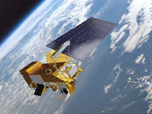
Jointly funded by NASA (National Aeronautics and Space Administration, USA), INPE (National Institute for Space Research, Brazil) and JAXA (Japan Aerospace Exploration Agency), Aqua (formerly known as EOS/PM-1) is part of NASA’s international Earth Observing System (EOS), as well as their Earth Science Enterprise (ESE) program. Aqua’s main focus is the multidisciplinary study of the Earth’s water cycle including cloud formation, precipitation, radiative properties, air-sea fluxes of energy, carbon and moisture, and sea ice concentrations and extents. Launched in May 2002 from Vandenberg Air Force Base, California, USA, Aqua had a design life of six years, however remains operational as of July 2022.
Quick facts
Overview
| Mission type | EO |
| Agency | JAXA, NASA, INPE |
| Mission status | Operational (extended) |
| Launch date | 04 May 2002 |
| Measurement domain | Atmosphere, Ocean, Land, Snow & Ice |
| Measurement category | Cloud type, amount and cloud top temperature, Liquid water and precipitation rate, Atmospheric Temperature Fields, Cloud particle properties and profile, Ocean colour/biology, Aerosols, Multi-purpose imagery (ocean), Radiation budget, Multi-purpose imagery (land), Surface temperature (land), Vegetation, Albedo and reflectance, Surface temperature (ocean), Atmospheric Humidity Fields, Ozone, Trace gases (excluding ozone), Sea ice cover, edge and thickness, Soil moisture, Snow cover, edge and depth, Ocean surface winds |
| Measurement detailed | Cloud top height, Ocean imagery and water leaving spectral radiance, Ocean chlorophyll concentration, Downward long-wave irradiance at Earth surface, Cloud cover, Cloud optical depth, Precipitation intensity at the surface (liquid or solid), Aerosol optical depth (column/profile), Cloud type, Cloud ice content (at cloud top), Color dissolved organic matter (CDOM), Cloud imagery, Cloud liquid water (column/profile), Land surface imagery, Upward short-wave irradiance at TOA, Upward long-wave irradiance at TOA, Cloud drop effective radius, Aerosol effective radius (column/profile), Fire temperature, Vegetation type, Fire fractional cover, Earth surface albedo, Downwelling (Incoming) solar radiation at TOA, Short-wave Earth surface bi-directional reflectance, Leaf Area Index (LAI), Land cover, Atmospheric specific humidity (column/profile), O3 Mole Fraction, Atmospheric temperature (column/profile), Land surface temperature, Sea surface temperature, CH4 Mole Fraction, Ocean suspended sediment concentration, Precipitation index (daily cumulative), Sea-ice cover, Snow cover, Soil moisture at the surface, Wind speed over sea surface (horizontal), Cloud top temperature, Normalized Differential Vegetation Index (NDVI), Snow water equivalent, Atmospheric stability index, Photosynthetically Active Radiation (PAR), Fraction of Absorbed PAR (FAPAR), CO2 Mole Fraction, CO Mole Fraction, Height of tropopause, Temperature of tropopause, Downward short-wave irradiance at Earth surface, Long-wave Earth surface emissivity, Diffuse attenuation coefficient (DAC), Upwelling (Outgoing) long-wave radiation at Earth surface, Short-wave cloud reflectance |
| Instruments | HSB, AIRS, AMSR-E, AMSU-A, CERES, MODIS |
| Instrument type | Imaging multi-spectral radiometers (vis/IR), Earth radiation budget radiometers, Imaging multi-spectral radiometers (passive microwave), Atmospheric temperature and humidity sounders |
| CEOS EO Handbook | See Aqua (EOS/PM-1) summary |
Summary
Mission Capabilities
Aqua has six instruments: the Atmospheric Infra-red Sounder (AIRS), the Advanced Microwave Scanning Radiometer-EOS (AMSR-E), the Advanced Microwave Sounding Unit-A (AMSU-A), the Cloud and the Earth’s Radiant Energy System (CERES), the Humidity Sounder for Brazil (HSB), and the Moderate-Resolution Imaging Spectroradiometer (MODIS).
The AIRS instrument is a medium resolution infrared spectrometer that provides high spectral resolution measurements of temperature and humidity profiles in the atmosphere. These include long-wave Earth surface emissivity, cloud diagnostics, surface temperatures and trace gas profiles. The instrument contains one infrared band and four near-infrared bands.
AMSU-A functions as an absorption-band microwave spectrometer that allows the satellite to capture all-weather night-day temperature sounding to an altitude of 45 km. HSB is also an absorption-band microwave spectrometer that records humidity soundings for climatological and atmospheric dynamics applications.
AMSR-E is a multi-purpose imaging microwave radiometer that attains measurements of water vapour, cloud liquid water, precipitation, winds, sea surface temperature, sea ice concentration, and soil moisture. The radiation measurements are collected via the CERES module and provide long term measurements of Earth’s radiation budget.
MODIS collects data on biological and physical processes on the Earth’s surface, in the lower atmosphere and on global dynamics, as well as surface temperatures of ocean and land processes, chlorophyll fluorescence, land and cloud cover.
Performance Specifications
AIRS contains more than 2300 spectral channels that have a spatial resolution of 0.4 - 14.4 μm, with an instantaneous field of view (IFOV) of 1.1°, field of view (FOV) of ± 49.5°, and swath width of 1650 km (13.5 km horizontal at nadir, 1km vertically positioned). The AMSU and HSB modules have a total of nineteen channels, with fifteen used by AMSU. AMSU is divided into two units, AMSU-A1 measures temperature profiles and has a swath width of approximately 1690 km, while AMSU-A2 is a smaller unit and has a nominal instantaneous field of view of 3.3°. The HSB module has a swath width of 1650 km with an IFOV of 1.1° or 13.5 km at nadir.
The AMSR-E instrument has a swath width of greater than 1450 km and an incidence angle of 55°. The instrument senses microwave radiation at 12 channels with 6 specific frequency ranges: 6.925, 10.65, 18.7, 23.8, 36.5 and 89.0 GHz. CERES has a resolution of 20 km and three specific channels of 0.3 - 5 um, 0.3 - 100 um, and 8 - 12 um. MODIS has a swath width of 2330 km and thirty-six bands in the range of 0.4 - 14.4 um.
Aqua is in sun-synchronous orbit at an altitude of 705 km with an orbital inclination of 98.2° and a repeat cycle of 16 days.
Space and Hardware Components
The Aqua spacecraft is based on the AB1200 bus design by TRW (now Northrop Grumman) and has a total mass of 2,934 kg. The propulsion system is a hydrazine blow-down system with four pairs of thrusters. The spacecraft had a design life of six years, which it has outlasted, and achieves radio-frequency communications based on the Consultative Committee for Space Data Systems (CCSDS) protocol and through Direct Broadcast (DB).
Aqua Mission (EOS/PM-1)
Spacecraft Launch Mission Status Sensor Complement References
The Aqua mission is a part of the NASA's international Earth Observing System (EOS). Aqua was formerly named EOS/PM-1, signifying its afternoon equatorial crossing time. NASA renamed the EOS/PM-1 satellite to Aqua on Oct. 18, 1999. The Aqua mission is part of NASA's ESE (Earth Science Enterprise) program. 1) 2) 3)
The focus of the Aqua mission is the multi-disciplinary study of the Earth's water cycle, including the interrelated processes (atmosphere, oceans, and land surface) and their relationship to Earth system changes. The data sets of Aqua provide information on cloud formation, precipitation, and radiative properties, air-sea fluxes of energy, carbon, and moisture (AIRS, AMSU, AMSR-E, HSB, CERES, MODIS); and sea ice concentrations and extents (AMSR-E).
Spacecraft
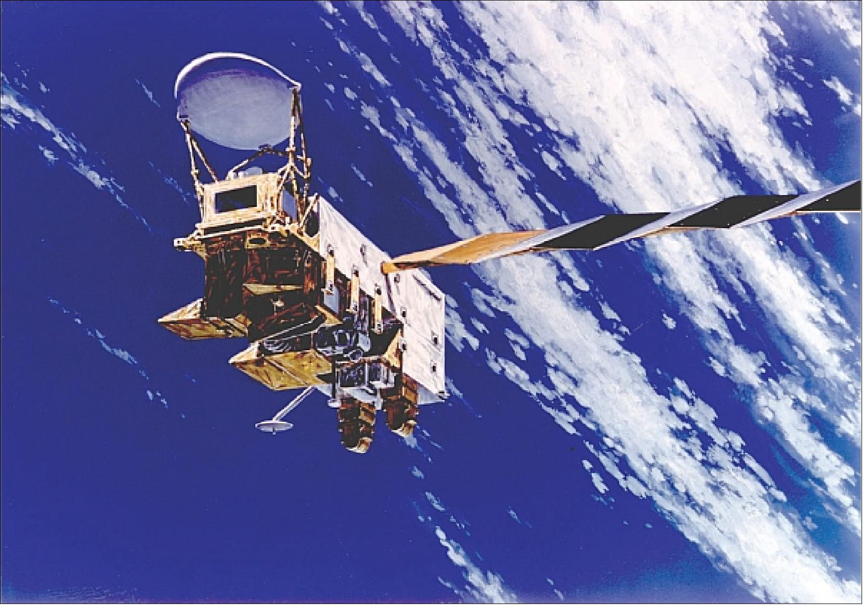
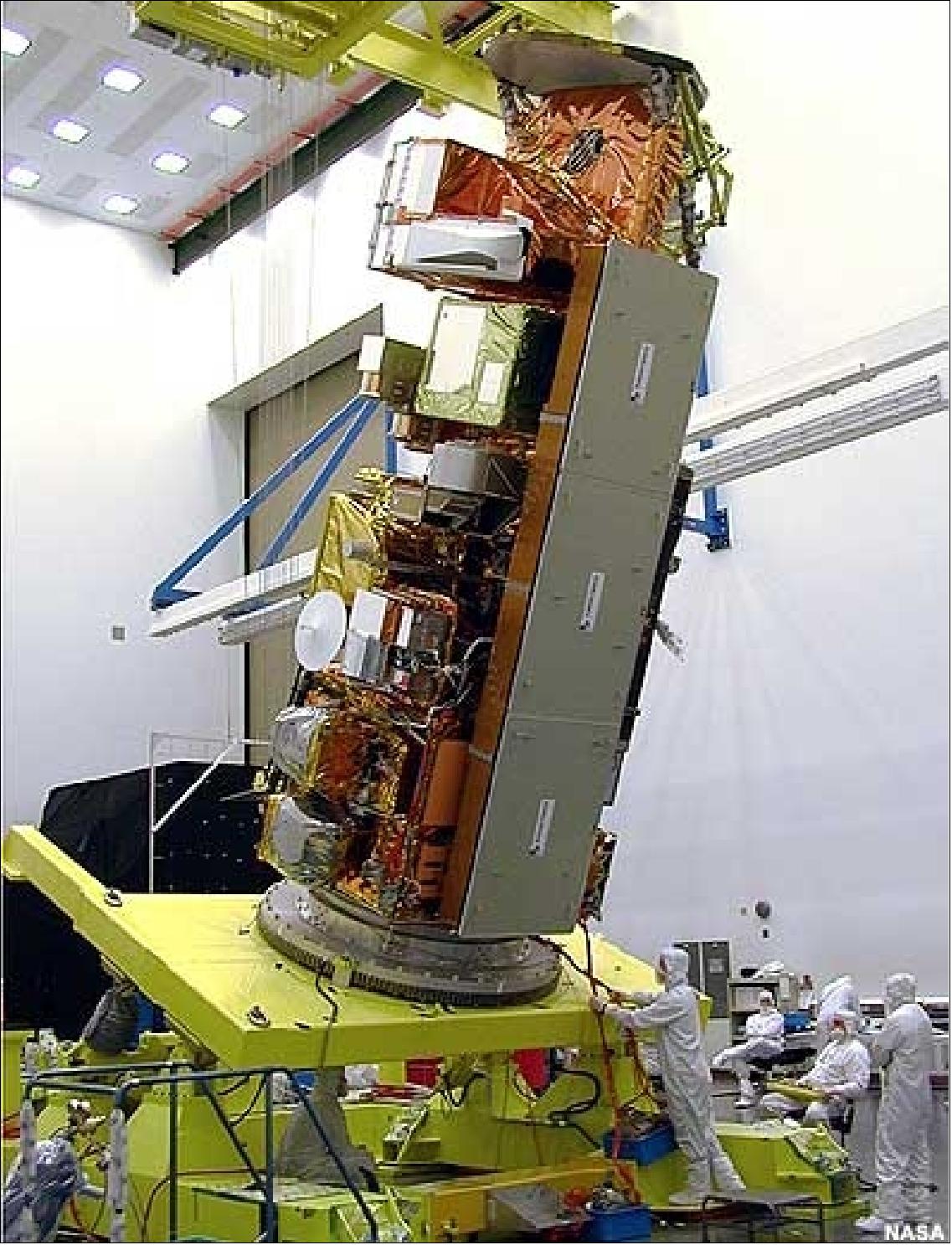
The Aqua spacecraft is based on TRW's modular, standardized AB1200 bus design (also referred to as T-330 platform) with common subsystems (Note: Northrop Grumman purchased TRW in Dec. 2002). The satellite dimensions are: 2.68 m x 2.47 m x 6.49 m (stowed) and 4.81 m x 16.70 m x 8.04 m (deployed). Aqua is three-axis stabilized, with a total mass of 2,934 kg at launch, S/C mass of 1,750 kg, payload mass =1,082 kg, propellant mass = 102 kg; power = 4.86 kW (EOL). Propulsion: hydrazine blow-down system; 4 pairs of thrusters. The design life is six years.
RF communications: X-band, S-band (TDRSS and Deep Space Network/Ground Network compatible). All communications are based on CCSDS protocols. Like the Terra mission, Aqua provides various means of payload data downlinks, among them Direct Broadcast (DB).
Launch
The Aqua spacecraft was launched on May 4, 2002 with a Delta-2 7920-10L vehicle from VAFB, CA. Aqua is the second satellite in NASA's series of EOS spacecraft. - Aura, the third of the three large satellites in the EOS series, was launched in July 2004 and is lined up behind Aqua, in the same orbit.
Orbit: Sun-synchronous circular orbit, altitude = 705 km (nominal), inclination = 98.2º, local equator crossing at 13:30 (1:30 PM) on ascending node, period = 98.8 minutes, the repeat cycle is 16 days (233 orbits).
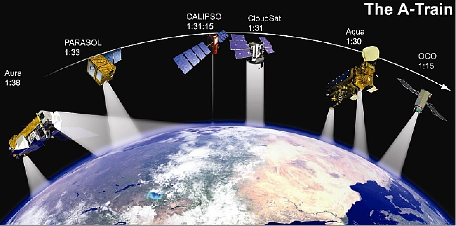
The Aqua spacecraft is part of the “A-train” (Aqua in the lead and Aura at the tail, the nominal separation between Aqua and Aura is about 15 minutes) or “afternoon constellation” (a loose formation flight which started sometime after the Aura launch July 15, 2004). The objective is to coordinate observations and to provide a coincident set of data on aerosol and cloud properties, radiative fluxes and atmospheric state essential for accurate quantification of aerosol and cloud radiative effects.
The PARASOL spacecraft of CNES (launch on Dec. 18, 2004) is part of the A-train as of February 2005. The OCO mission (launch in 2009) will be the newest member of the A-train. Once completed, the A-train will be led by OCO, followed by Aqua, then CloudSat, CALIPSO, PARASOL, and, in the rear, Aura. 4)
Note: The OCO (Orbiting Carbon Observatory) spacecraft experienced a launch failure on Feb. 24, 2009 - hence, it is not part of the A-train.
Note: As of 19 April 2022, the previously single large Aqua file has been split into three files, to make the file handling manageable for all parties concerned, in particular for the user community.
• This article covers the Aqua mission and its imagery in the period 2022
• Aqua imagery in the period 2021-2020
• Aqua imagery in the period 2019-2002
Mission Status
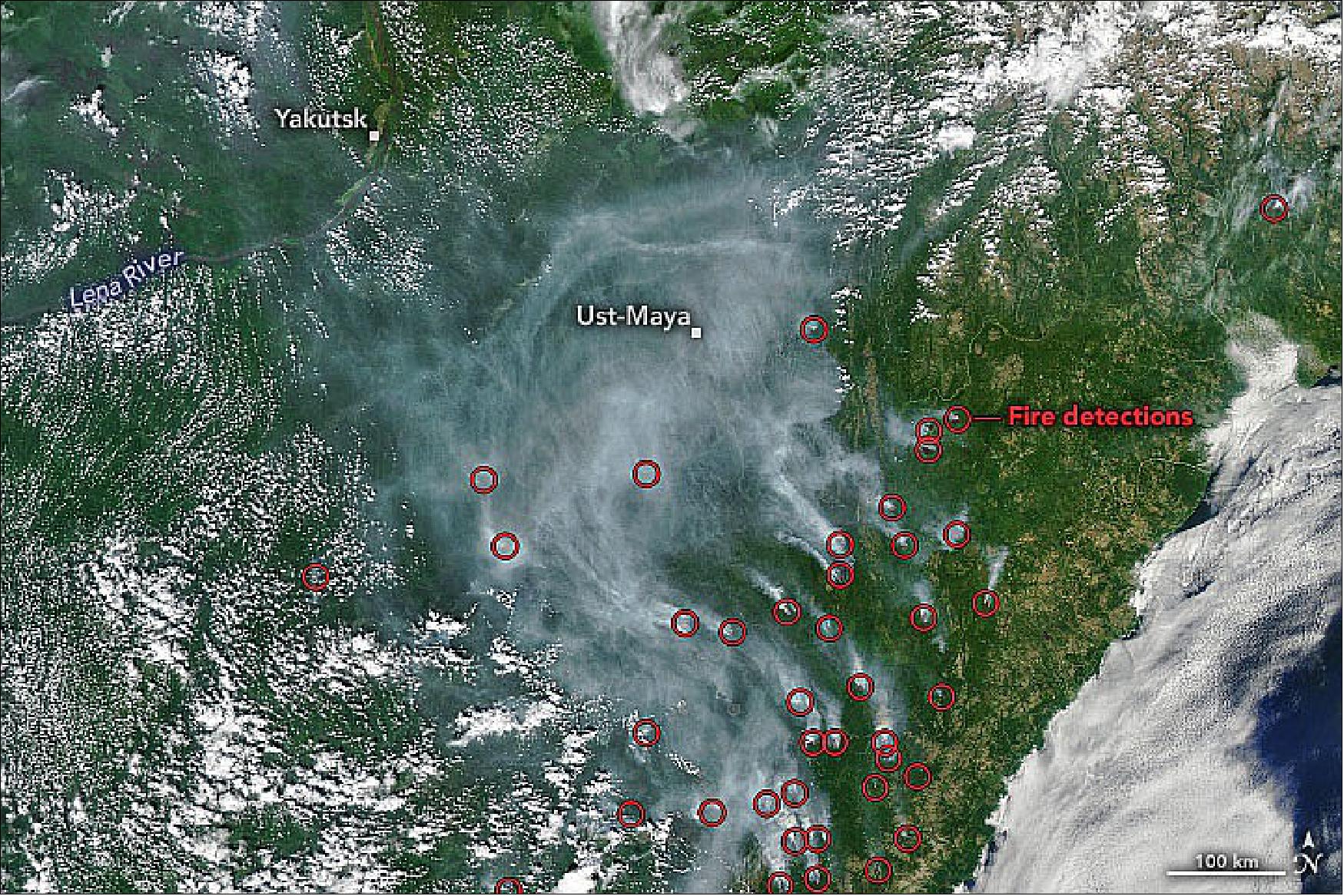
• July 19, 2022: During the first week of July, NASA satellites began detecting signs that several wildland fires were burning in Russia’s far east. Two weeks later, several fires had grown much larger and more intense, creating rivers of smoke that flowed over parts of Khabarovsk and the neighboring Republic of Sakha (Yakutia). 5)
- According to Sakha’s emergencies ministry, 51 fires burned across roughly 9,737 hectares (38 square miles) on July 18. More than 500 people were fighting the fires in Sakha, and thousands more were deployed to fire fronts across Russia, according to Russia’s ministry of emergency situations (EMERCOM).
- For the past two years, Sakha has endured unusually severe fire seasons. In 2021, more than 8.4 million hectares (84,000 km2) of forests burned in Sakha, nearly four times the long-term average.
- Fires are not the only hazard facing the region. Flooding along the Yana River recently displaced hundreds of people in Sakha.
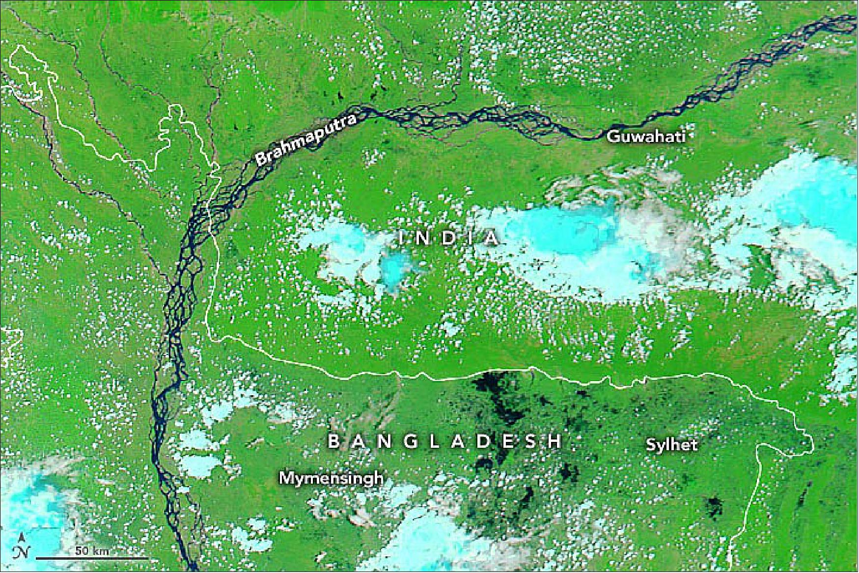
• June 24, 2022: Torrential monsoon rains, lightning, and landslides are common in Bangladesh and the northeastern Indian states of Assam and Meghalaya during the summer. But the intensity of the severe weather that pummeled the low-lying region in mid-June 2022 stands out. 6)
- After weeks of downpours, flooding has swamped millions of homes and displaced hundreds of thousands of people in India and Bangladesh, according to reports from humanitarian agencies. Officials from the hard-hit Sylhet region of Bangladesh have called the floods the worst to hit the area in more than a century.
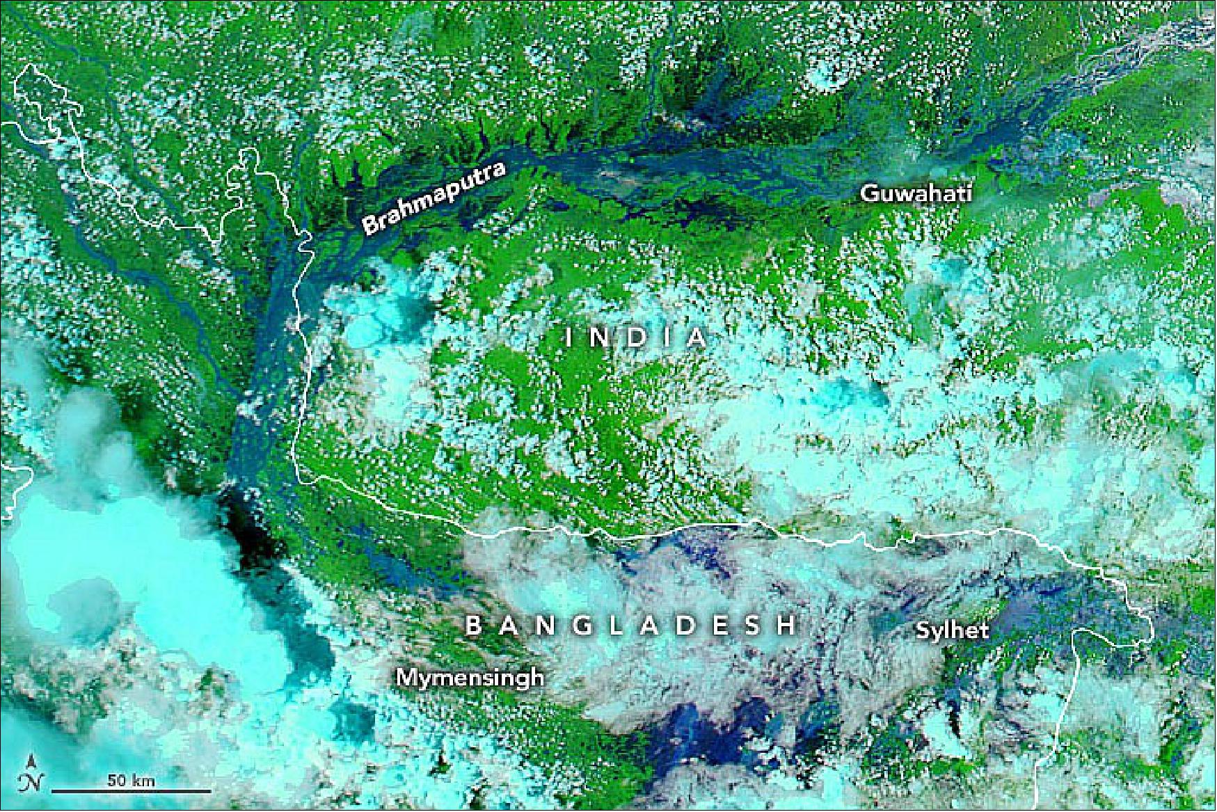
- On June 22, the Bangladesh Flood Forecasting and Warning Centre reported water levels along the Surma River in Sylhet were at or above “danger level” at several locations. About half of the croplands in Sylhet have been flooded, according to the Dhaka Times.
• June 15, 2022: On June 4–5, 2022, thunderstorms moved across south-central and southwest Alaska, delivering nearly 5,000 lightning strikes and igniting dozens of wildfires. It was the latest outbreak in an unusually active fire season so far. 7)
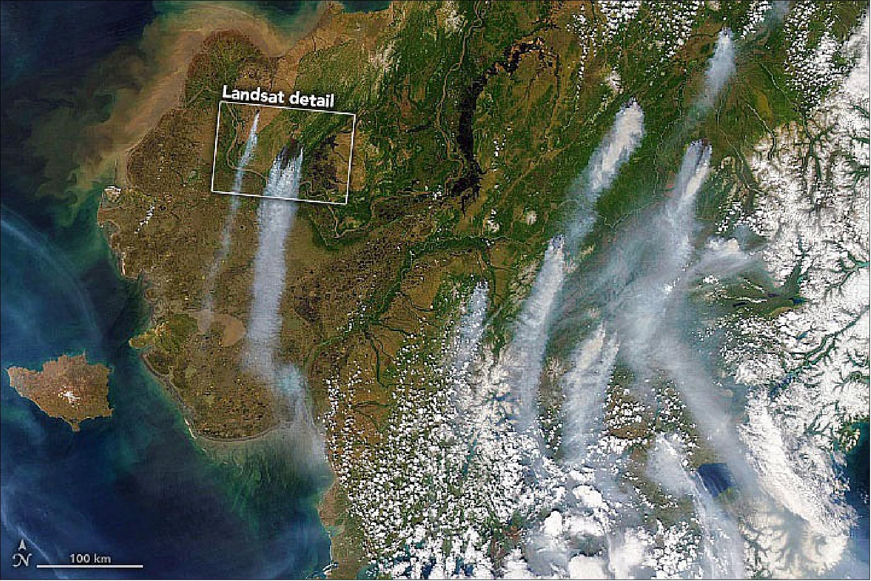
- In the Yukon Delta, the East Fork fire has become the largest tundra fire on record. Ignited on May 31 by a lightning strike, it has burned more than 150,000 acres along the Yukon River north of the village of St. Mary’s.

- Northerly winds drove the East Fork fire within about 3.5 miles (6 km) of the village of St. Mary’s. Although no mandatory evacuation orders were issued, residents of St. Mary’s, and the nearby Yukon River villages of Mountain Village, Pitkas Point, and Pilot Station—all of which can be reached only by boat or plane—were encouraged to voluntarily relocate.
- On June 13, the wind shifted and allowed firefighters to attack the western edge of the fire. The firefighters were supported by “scooper” aircraft dropping water, and by drones dropping ping-pong sized plastic balls that ignite to burn vegetation and create fire breaks.
- To the east, the Hog Butte fire has so far burned about 58,000 acres about 125 miles (200 kilometers) west of Denali National Park. On June 11, 2022, the Hog Butte fire spawned a pyrocumulonimbus cloud (pyroCb) that reached an altitude of about 6 miles (10 kilometers). It was the first pyroCb over Alaska in two years.
- According to a report from the Alaska Interagency Coordination Center, by mid-June this year, 250 wildfires had already burned more than 770,000 acres, not counting prescribed burns. That is already more than the 30-year median of 600,000 acres burned during the entire wildfire season, noted Rick Thoman, a climate specialist at the Alaska Center for Climate Assessment & Policy and the International Arctic Research Center at the University of Alaska Fairbanks. Over the last 30 years, the median area burned by mid-June has been about 50,000 acres.
- Smoke from the wildfires drifted over the Alaska Range into Anchorage and northeast across the state causing reduced visibility and poor air quality.
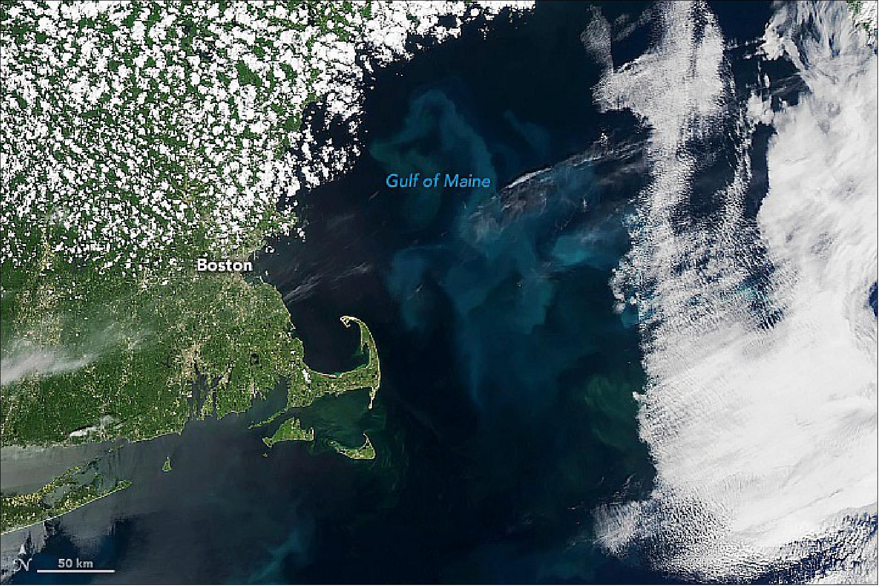
• June 8, 2022: The Gulf of Maine is growing warmer and saltier, and those changes have led to a substantial decrease in the productivity of phytoplankton that are the center of the marine food web. Specifically, phytoplankton in the gulf are now about 65 percent less productive than they were two decades ago, scientists from Bigelow Laboratory for Ocean Sciences reported in research published on June 7, 2022. 8)
- The Gulf of Maine helps fuel New England’s marine ecosystems and maritime economy. Like plants on land, phytoplankton absorb carbon dioxide from the atmosphere and use sunlight to grow via photosynthesis; they then become food for other organisms. Disruptions to the productivity of these microscopic organisms can lead to adverse effects on the region’s fisheries and the communities that depend on them.
- Research published in 2021 showed that the Gulf of Maine has been warming faster than most ocean basins. In the new effort from Bigelow, funded in part by NASA, scientists showed how that warming has affected the phytoplankton.
- “Phytoplankton are at the base of the marine food web on which all of life in the ocean depends, so it’s incredibly significant that its productivity has decreased,” said William Balch, a Bigelow Laboratory scientist who co-led the study. “A drop of 65 percent will undoubtedly have an effect on the carbon flowing through the marine food web, through phytoplankton-eating zooplankton, and up to fish and apex predators.”
- The findings are the result of an analysis of the Gulf of Maine North Atlantic Time Series (GNATS), a 23-year sampling program that has measured the temperature, salinity, and other chemical, biological, and optical properties of the gulf. Balch says the changes that they are recording show an intricate connection between the gulf and the greater Atlantic Ocean.
- “It’s all being driven by this gigantic windmill effect happening out in the North Atlantic, which is also changing the circulation coming into the Gulf of Maine,” Balch explained. “There used to be these inflows from the North Atlantic bringing water from the southward-flowing Labrador Current, making the gulf cooler and fresher, as opposed to warmer and saltier, which is where we are now.”
- Since 1998, Bigelow Laboratory has tracked biogeochemical changes in the gulf by collecting water samples via commercial ferries and research vessels cruising along the same routes repeatedly. They also use autonomous gliders that cross the same sampling lines.
- Such in situ measurements are critical for making sure satellite observations are accurate and for filling in gaps on days when skies are cloudy or foggy. NASA acquires ocean color data through Aqua, Terra, and other satellites. The upcoming Plankton, Aerosol, Cloud, ocean Ecosystem (PACE) mission is expected to significantly improve and extend observations of the many colors of the ocean associated with different types and concentrations of phytoplankton.
- “We are focused very much on that lower level, the phytoplankton level,” said Bigelow Laboratory scientist and project co-lead Catherine Mitchell. “But the changes at that level can have all these implications at the higher species, the fisheries, the lobster, and all those kinds of industries that are important within the state of Maine and other states that border the gulf.”
- “If you're trying to look at something like climate change,” Balch added, “the statistical power of sampling over and over again the same exact water masses is really powerful stuff.” The GNATS dataset is available for scientific, commercial, and educational purposes via NASA’s repository for in situ oceanographic and atmospheric data.
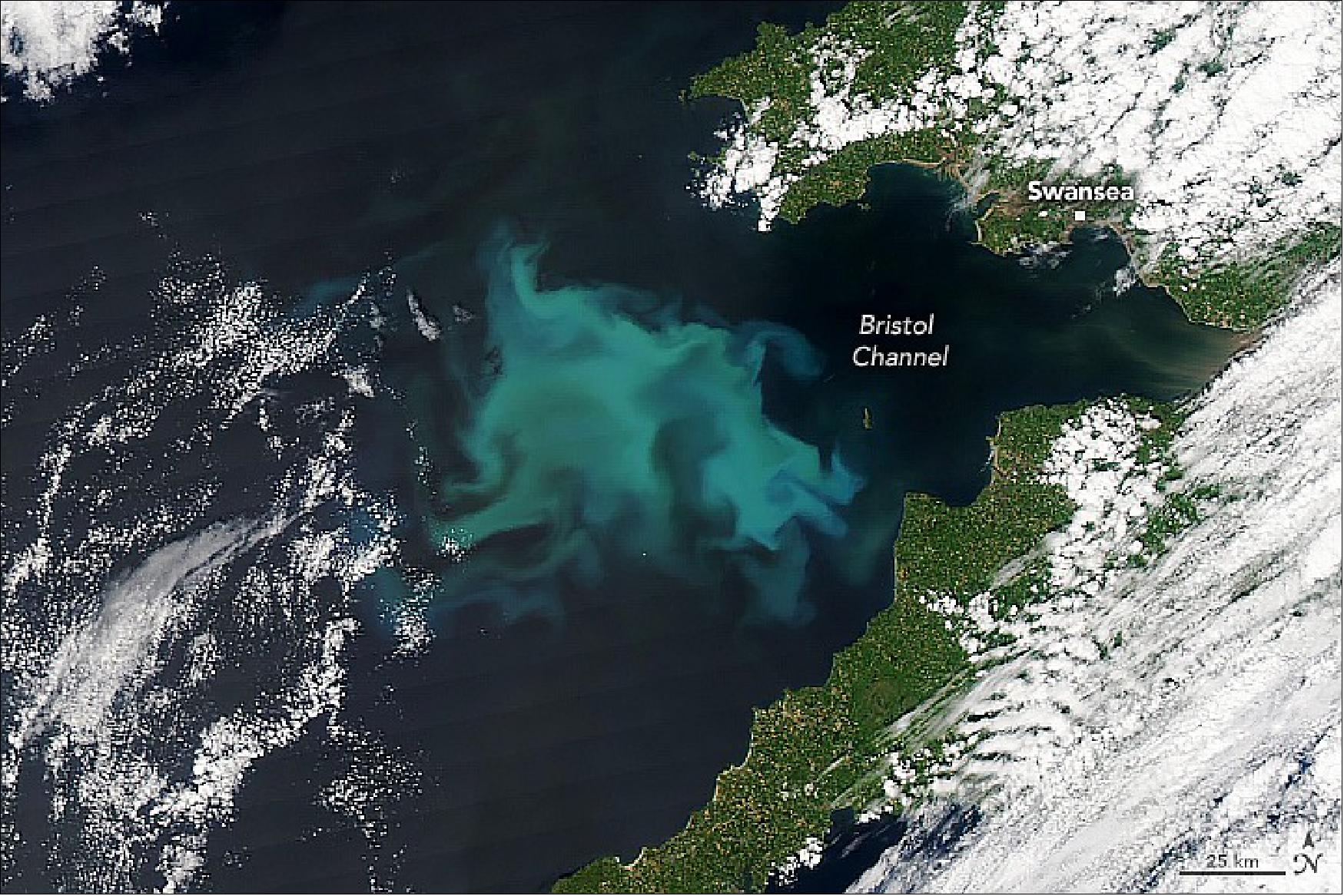
• June 4, 2022: Early summer blooms colored the seas off of southern Wales and southwestern England when NASA’s Aqua satellite passed over the region on June 3, 2022. Bright blue-green waters indicated an abundance of phytoplankton just beyond Bristol Channel. 9)
- Phytoplankton are usually most abundant in the far North Atlantic and the North Sea in late spring and early summer, when dissolved nutrient levels are high. Melting snow and ice and spring rains bring increased runoff into the sea, often bearing a heavy load of sediment and organic matter while freshening surface waters. Recent Sahara dust storms also may have dropped nutrients into the sea here. Increasing seasonal sunlight provides the fuel for growth.
- The milky, light-colored waters are likely filled with coccolithophores, phytoplankton with calcium carbonate plates that appear chalky white when amassed in great numbers. Greener patches may be rich with diatoms. It is impossible to know for sure without taking direct water samples.
- Phytoplankton are microscopic, plant-like organisms that float near the ocean surface and turn sunlight and carbon dioxide into sugars and oxygen. In turn, they become food for the grazing zooplankton, shellfish, and finfish. They also play an important but not fully understood role in the global carbon cycle, taking carbon dioxide out of the atmosphere and eventually sinking it to the bottom of the ocean.
- Bristol Channel is the largest natural inlet of the United Kingdom. Freshwater from the River Severn (the UK’s longest) pours into an estuary here and mixes sediment and nutrients into the saltwater. Populations of pollock, whiting, bass, and eels are known to congregate here, as well as several species of porpoises, dolphins, sharks, crabs, and cockles.
- In a recent study led by Abigail McQuatters-Gollop of Plymouth University, scientists reported that the types and abundances of plankton in the waters around the United Kingdom have changed significantly in the past six decades. The shifts are likely related to climate change—particularly warming temperatures—and could have long-term effects on the health and distribution of fish, marine mammals, and sea birds in the region. 10)
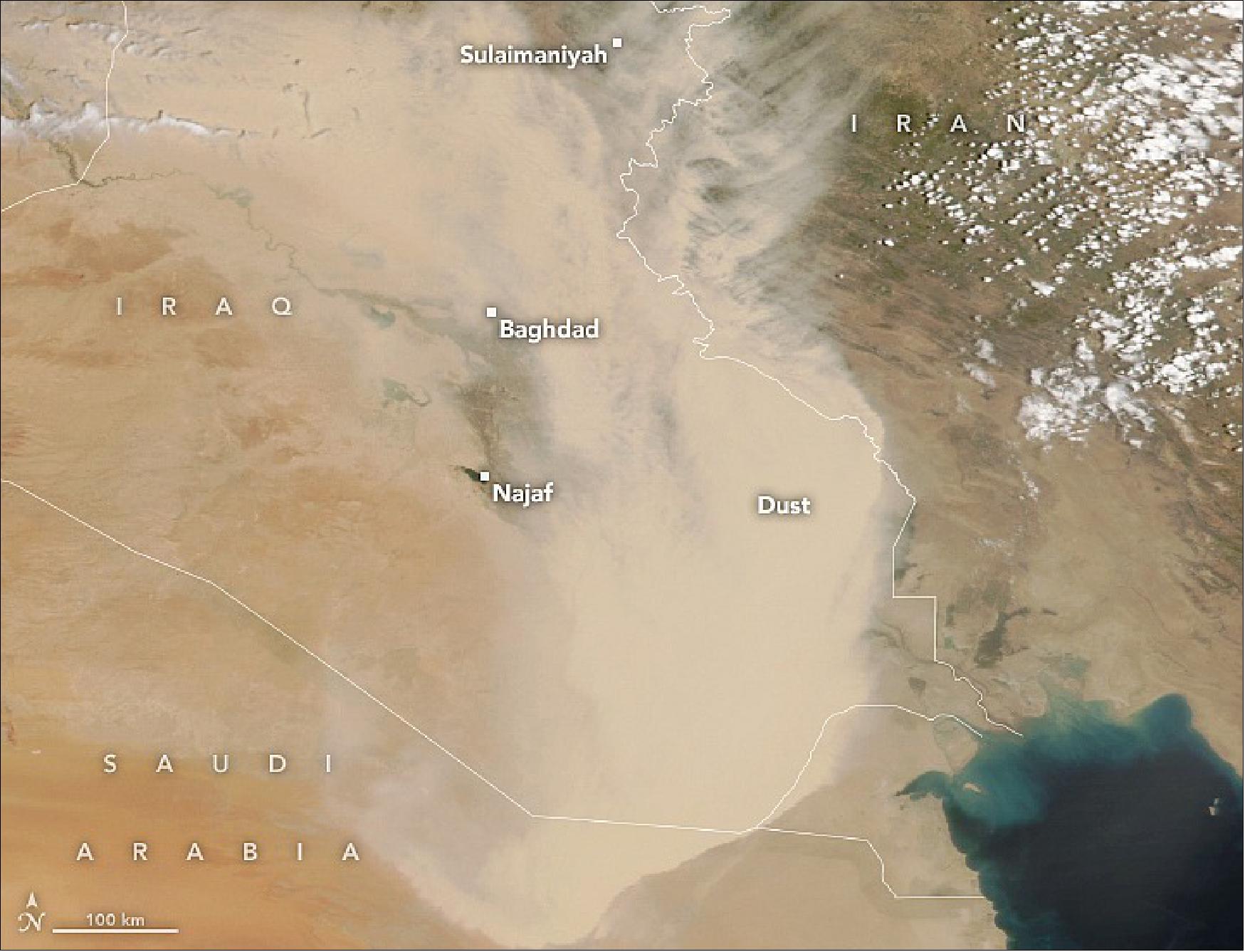
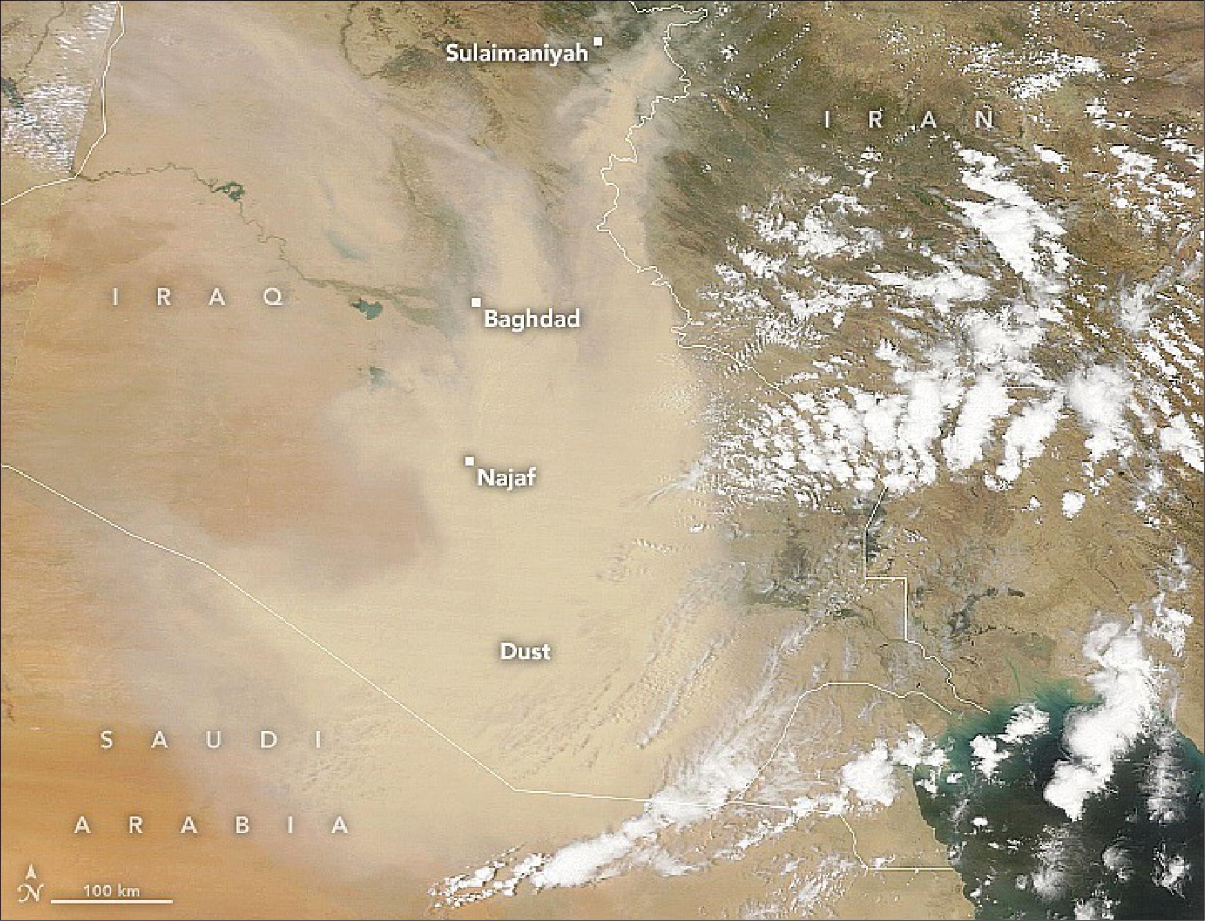
• May 18, 2022: Since the beginning of April 2022, Iraq and other parts of the Middle East have been hit by a series of severe dust storms. Two major storms in the past two weeks have sent thousands of people to the hospital, as poor air quality from airborne dust can aggravate asthma and other respiratory diseases. 11)
- The skies above Baghdad, Najaf, Sulaimaniyah, and other cities turned orange as visibility dropped to a few hundred meters. Several airports were closed during the dust events, and schools were closed nationwide. Government offices were shuttered in seven of the Iraq’s 18 provinces, and several governors declared states of emergency.
- Dust storms in Iraq are most common in late spring and summer, provoked by seasonal winds such as the “shamal” that blows in from the northwest. Researchers suggested in a 2016 paper that La Niña conditions in the equatorial Pacific can lead to an earlier onset of shamal winds. Recent observations suggest that La Niña may be persisting into a third consecutive year.
- Those strong seasonal winds blow across abundant sources of dust. According to The World Bank, northern Iraq—between the Tigris and Euphrates rivers—has the highest density of dust sources in the Middle East.
- News media reported that Iraq has been hit by at least eight dust storms in the past six weeks. Researchers have found that dust events have become more frequent in Iraq. The country has been facing drought conditions in recent years, as well as land-use changes and overuse that mean there is more loose soil available to be lofted into the atmosphere. The World Bank cited Iraq as one of the countries most vulnerable to desertification and climate change.
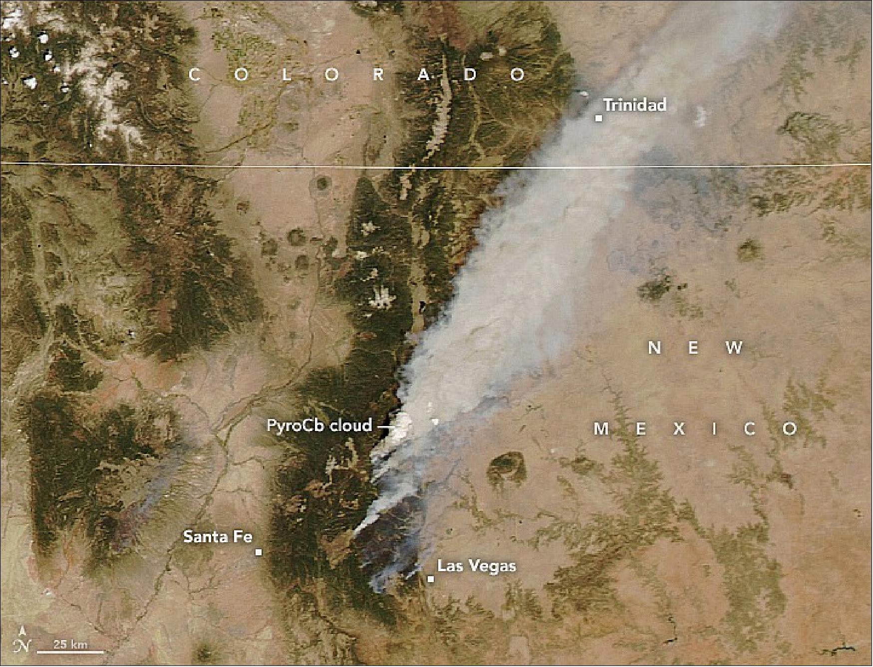
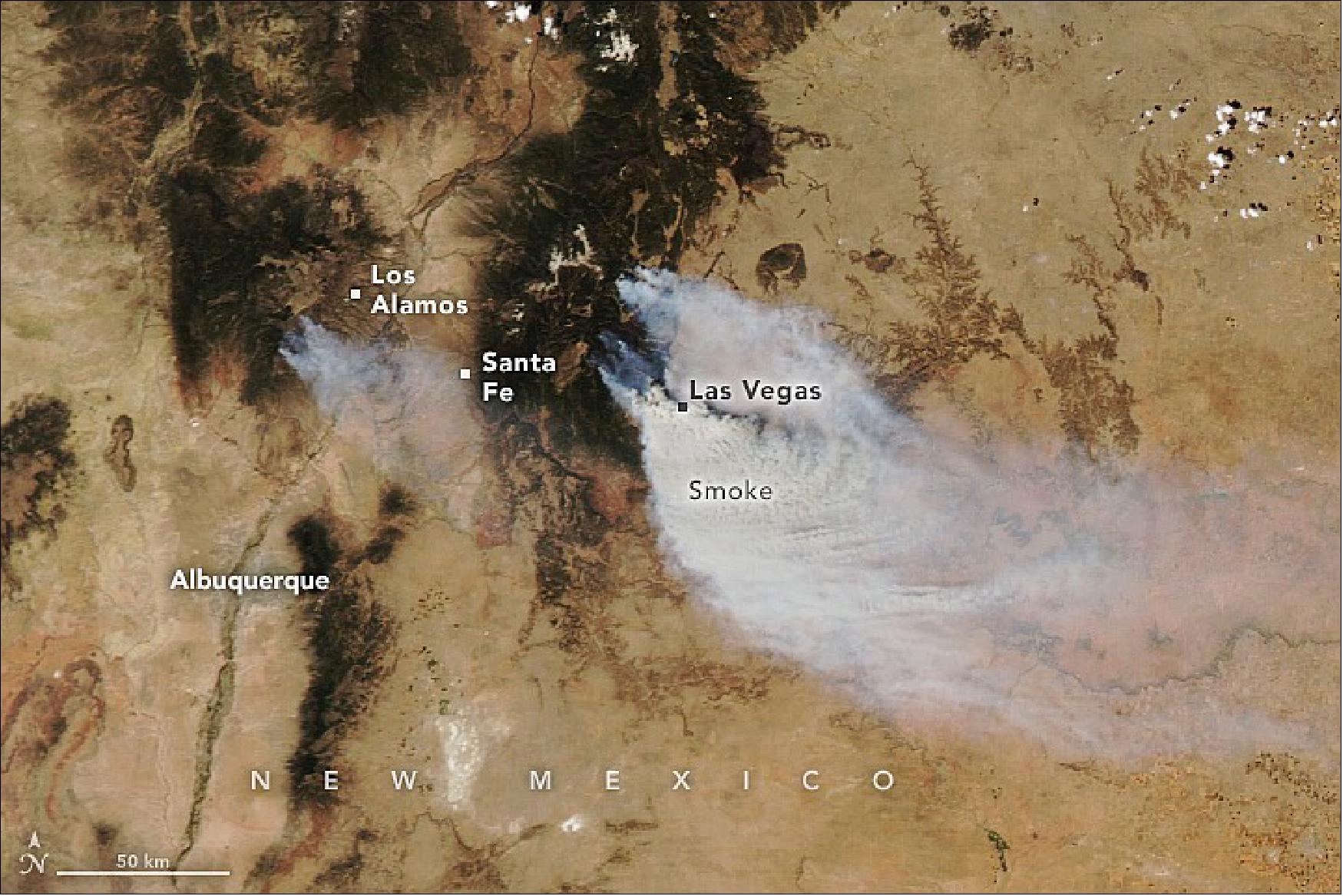
• May 14, 2022: The Calf Canyon-Hermits Peak fire continued to rage across northern New Mexico in mid-May 2022, entering its second month. On May 13, it was the largest fire burning in the United States and the second largest in New Mexico’s history. 12)
- The burned area spanned more than 270,000 acres east of Santa Fe and stretched 50 miles (80 km) from its northern to southern perimeter in the Sangre de Cristo mountains. As of May 13, the fire was 29 percent contained, mostly on its southern perimeter, but continued to spread northeast. Hundreds of buildings and homes have been destroyed, and thousands of people were evacuated. Evacuation orders remained in effect in San Miguel, Moro, and Colfax counties, and have been expanded into the ski resort town of Angel Fire.
- Periods of critical fire weather continued to challenge the 1,800 firefighters battling the blaze. Extremely low humidity and high winds helped spread the fire through dry grass, brush, and trees. Periodic gusts reaching 65 miles (105 km) per hour prevented aerial firefighting efforts, including water drops and the dispersal of flame retardant.
- Researchers at the Cooperative Institute for Meteorological Satellite Studies measured a cloud-top temperature of -59°C (-75°F). This indicated that the cloud had reached the tropopause, the boundary between the troposphere and the stratosphere at an altitude of about 12 km.
- “This is considered to be a small pyroCb,” said Mike Fromm, a meteorologist with the U.S. Naval Research Laboratory. “The significance is that it is still early in the fire season, so any indication of such a blowup tells us to be on high alert for more and bigger pyroCb events.”
- The Calf Canyon-Hermits Peak fire complex formed when two smaller fires merged on April 22-23. The Hermits Peak fire had started as a prescribed burn in part of the Santa Fe National Forest on April 6, but erratic, gusty winds blew it out of control. The cause of the Calf Canyon fire, which started on April 19, is still being investigated.
- Several other large fires also continued to burn across New Mexico in mid-May. The Cerro Pelado Fire burning southwest of Los Alamos National Laboratory has surpassed 45,000 acres and is 19% contained. The Cooks Peak Fire has burned 60,000 acres north of Las Vegas, New Mexico, and was 97% contained on May 13. Smoke from the fires has drifted north into Colorado and northeast across Kansas and the Midwest.
- Most of the state continues to experience extreme to exceptional drought in the midst of the Southwest megadrought. New Mexico has had 244 fires so far this year, burning more than 360,000 acres, according to the National Interagency Fire Center. That is roughly three times as much acreage as was burned in 2021, when 672 fires burned about 124,000 acres.
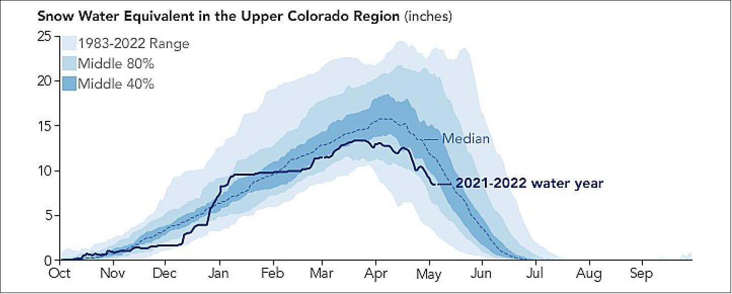
• May 6, 2022: As another winter ends with the U.S. West still in the grip of the worst megadrought in 1,200 years, scientists and water managers are looking at the state of the snowpack. Mountain snowpack is a natural reservoir: As it melts out over the course of the spring and summer, it provides a steady supply of water for millions of people who rely upon it for agriculture, industry, and municipal and residential use. 13) 14)
- To forecast water supplies for the coming year, hydrologists and water managers rely on measurements of snowpack, particularly the snow water equivalent (SWE), a measure of how much liquid water is stored within snow. In the western U.S., snowpacks usually peak around April 1. Assessment of the snowpack on this date has traditionally been used to help predict streamflows, reservoir storage levels, and potential wildfire conditions for the rest of the year.
- This year, with drought-related moisture deficits in the soil and atmosphere, researchers are seeing widespread and severe low-snow and low-runoff conditions across the West, said Benjamin Hatchett, a hydroclimatologist at the Desert Research Institute who studies snow droughts. “Usually, some regions will be bad, some will be doing okay, and others will be doing great,” Hatchett noted. “But when everywhere [in the West] is in this low-snow condition, it’s pretty concerning.”
- While satellites can show where snow is, they cannot yet directly measure snow depth or snow water equivalents. Measurements of snow have been made manually since the early 1900s. In the late 1970s, automated ground-based monitoring began with the SNOTEL network, which is managed by the Department of Agriculture’s Natural Resources Conservation Service. The network is composed of more than 900 monitoring stations placed in remote, high-elevation watersheds in the western U.S., where automated instruments measure snowpack, precipitation, temperature, and other climate conditions.
- SNOTEL stations record data at a single point location, mostly within a narrow high-elevation range. To estimate the snowpack between and beyond the stations—such as higher elevations and wider geographic areas—researchers must extrapolate and interpolate.
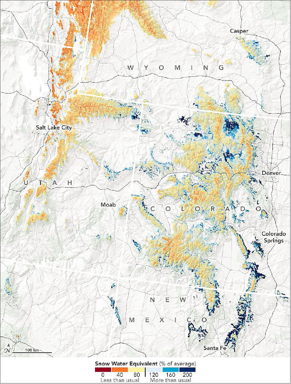
- Researchers at the Institute of Arctic and Alpine Research (INSTAAR) at the University of Colorado (CU) Boulder are looking to satellite data to improve those estimates of snow water equivalent. Noah Molotch, an INSTAAR hydrologist with a joint appointment at NASA’s Jet Propulsion Laboratory, and CU-Boulder colleague Leanne Lestak have been using 20 years of satellite data of snow-covered area, along with the SNOTEL data, to generate close to real-time estimates of SWE for use by the U.S. Bureau of Reclamation. Their modeling effort can fill the gaps that ground monitoring doesn’t cover, particularly at certain elevations.
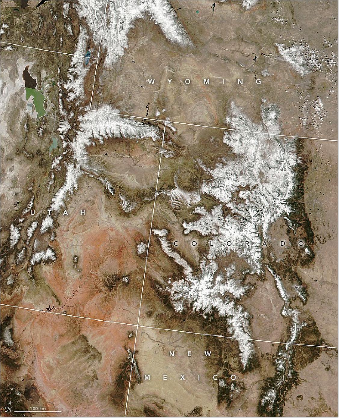
- Despite some pockets of anomalously high SWE (Snow Water Equivalent), most areas range from 46 to 95 percent of the 2000–2020 average. Data on the snow-covered area come from Moderate Resolution Imaging Spectroradiometer (MODIS) on NASA’s Terra satellite. The model also accounts for variables such as elevation, slope, latitude, and upwind mountain barriers, as well as historical patterns of SWE and melting dates.
- “Water managers really like to see how much snow there is and what the percentage average is at different elevation bands,” said Molotch. “That’s where actually the spatial product is really valuable. Water managers know that snow from low elevations will run off earlier and increase stream flow early in the season, whereas higher elevations run off later and will be the primary source of streamflow later.”
- In an April 18 report issued by the Colorado Basin River Forecast Center, forecasters predicted a near-average to much-below average water supply volume for April to July 2022 across the Upper Colorado River Basin and Great Basin.
- The Colorado River basin covers an area of 246,000 square miles (637,000 km2). This drainage supplies water to tens of millions of people, including those in large urban areas outside the basin, like Denver, Salt Lake City, and Los Angeles, who receive water through diversion projects like tunnels and canals. When snow melts and the water makes it to the Colorado River, it is collected and stored in Lake Mead behind Hoover Dam and in Lake Powell behind Glen Canyon Dam. Hydropower generated at Glen Canyon alone provides electricity to about 5 million people in seven states.
- Lake Powell has dropped to its lowest level since the reservoir was first filled in the 1960s. Water behind the dam stands at 3,522 feet9 above sea level or 24 percent of capacity. If the water drops to a critical level of 3,490 feet, the dam’s ability to produce hydropower will be threatened. On May 3, the U.S. Bureau of Reclamation announced that it will take action to maintain critical hydropower-generating capacity at Lake Powell. Over the next 12 months, the agency will allow more water to flow into the lake from upstream reservoirs and less water to be released downstream.
• May 5, 2022: On April 13, a blizzard dropped 4 feet of snow on Minot, North Dakota, as a drought-fueled wildfire burned in Ruidoso, New Mexico, and severe storms spawned eight tornadoes in Kentucky. NASA’s Atmospheric Infrared Sounder (AIRS) helped weather forecasters predict these events, as it’s been doing since it was launched in 2002. But now AIRS also helps researchers calculate the role climate change plays in these extreme weather events. It has become indispensable in other ways that couldn’t be foreseen when the weather instrument launched aboard NASA’s Aqua satellite in May 2002. 15)
- “Understanding what happened in the first couple of decades of the 21st century is critical to understanding climate change, and there’s no better record than AIRS to study that,” said Joao Teixeira, AIRS science team leader at NASA’s Jet Propulsion Laboratory in Southern California. “I see us as guardians of this precious dataset that will be our legacy for future generations.”
- AIRS measures infrared – heat – radiation from the air below the satellite to create three-dimensional maps of atmospheric temperature and water vapor, the main ingredients for any kind of weather. The instrument proved to be an almost immediate success: Within three years after AIRS’ launch, assessments of forecasts made by professional meteorologists showed that incorporating AIRS data in weather forecasting models produced a significant increase in accuracy.
Looking Beyond Weather
- The AIRS instrument is a spectrometer that breaks radiation into wavelengths, just as a prism does. But where earlier spectrometers in space had 15 or 20 detectors that each observed broad bands of infrared wavelengths, AIRS has 2,378 detectors that each senses a specific wavelength, and every detector makes close to 3 million measurements a day. This enormous advance in data quality and quantity not only succeeded in improving weather forecasting, but inspired a new generation of similar spaceborne instruments from space agencies around the world.
- In 2002, getting this technology ready to launch required an innovative design and skillful construction to accommodate the thousands of detectors. The instrument’s creators eventually arranged the detectors in 17 long lines, each of them two detectors wide (for redundancy in case one failed) by about 150 detectors long, and packaged them onto a single focal plane assembly. “When I first saw it, I said, ‘You’ve got to be kidding me,’” said Tom Pagano, AIRS’ project manager at JPL. “It was a major engineering achievement for the time.” Other advances, like the development of a frictionless cryocooler to cool AIRS’ detectors, led to an instrument that has lasted an extremely long time and is extraordinarily stable.
- “Due to the amazing engineering, the data we have now is almost the same quality as it was 20 years ago, when the instrument was new,” Teixeira said.
- Stability is essential for scientists to pinpoint the small but persistent signals of climate change from out of the noise of year-to-year variations in weather. As the global temperature creeps upward toward 1.5 degrees Celsius higher than pre-industrial times, AIRS’ two decades of consistent and multifaceted measurements provide a satellite record of global warming that is second to none. There are other satellite records of individual greenhouse gases or of surface temperature, for example, but no other global data record matches the time span and wide range of wavelengths in the AIRS dataset.
Legacy Building
- When AIRS launched, the mission team aspired to collect data for 15 years, said Pagano. “We put an unimaginable amount of effort into making an instrument that wouldn’t fail in orbit. It was the philosophy of how we built these instruments on the Aqua satellite.”
- And as the data has kept coming, researchers have found more and more uses for it. Researchers recently used AIRS data to detect atmospheric waves from the eruption of the Hunga Tonga-Hunga Ha’apai volcano. Earlier this year, researchers also used AIRS data to quantify the link between humidity and influenza outbreaks. In addition, AIRS data is used to track clouds, carbon dioxide, methane, ozone, and other gases and pollutants whose spectral signatures fall within the range of infrared wavelengths AIRS detects.
- The AIRS team and other researchers are still looking into even more applications of the dataset. “There’s more to mine from this instrument,” Pagano said. “It has such rich information content.”
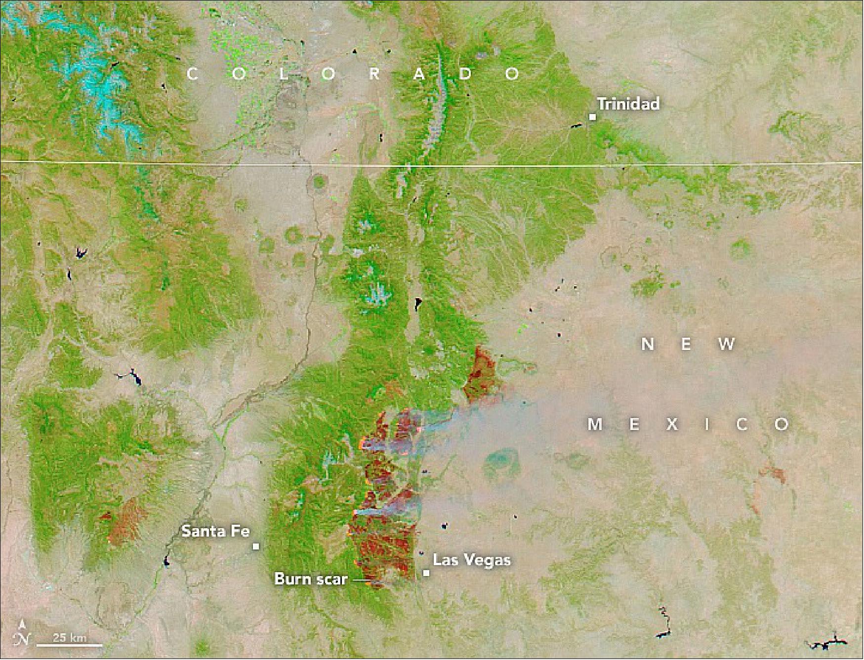
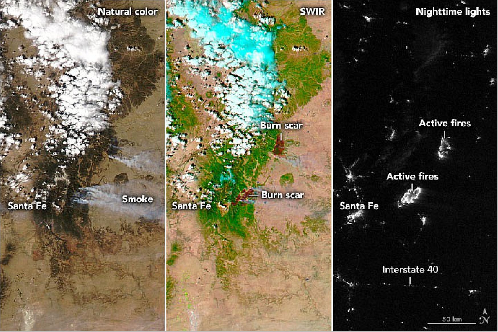
• May 4, 2022: Early season wildfires continued to rage in the first week of May 2022 in northern New Mexico. The blazes have been driven by high winds, low humidity, and exceptionally dry tinder—grass, brush, and timber—that are providing ample fuel for burning. The fires have destroyed hundreds of structures and prompted the evacuation of thousands of homes. On May 3, 2022, seven large fires were still burning across the state. 16)
- Earlier in the week, a few days of cooler, slightly more humid weather provided a brief respite before drier, windier conditions brought red flag warnings back to the state. More than a thousand firefighters are battling the Calf Canyon-Hermits Peak fire, two fires that merged on April 22-23 to form one of the largest wildfires in state history.
- As of May 3, the Calf Canyon-Hermits Peak complex had burned more than 145,000 acres northwest of the historic town of town of Las Vegas, New Mexico; the fire was 20 percent contained. The Hermits Peak fire started as a prescribed burn in part of the Santa Fe National Forest on April 6, but erratic, gusty winds blew it out of control.
- The Cerro Pelado fire burning southwest of Los Alamos started on April 22 and quickly spread across 5,000 acres, prompting evacuations of some nearby communities. As of May 3, the fire had burned more than 25,000 acres and was 10 percent contained. Incident commanders predicted extreme fire behavior to continue as high winds pushed the fire into extremely dry fuels to the northeast and southeast. As of May 2, the fire was burning about 10 km (6 miles) southwest of Los Alamos National Laboratory. Nearby Valles Caldera National Preserve and Bandelier National Monument were closed until further notice.
- About 80 km (50 miles) north of Las Vegas, the 60,000-acre Cooks Peak fire, which started on April 17, was 72 percent contained on May 3.
- According to the U.S. Drought Monitor on April 26, 2022, approximately 99 percent of the state was experiencing drought, with 83 percent facing extreme to exceptional dryness. New Mexico has had 211 fires so far this year, burning a total of 230,000 acres. In all of 2021, 672 fires burned nearly 124,000 acres, according to the National Interagency Fire Center.
- MODIS sensors have also imaged burn scars from the New Mexico fires. Many NASA satellites and instruments are used to detect actively burning fires, track the transport of smoke, provide information for fire managers, and map the extent and severity of burn scars. Satellites are often the first to detect wildfires in remote regions.
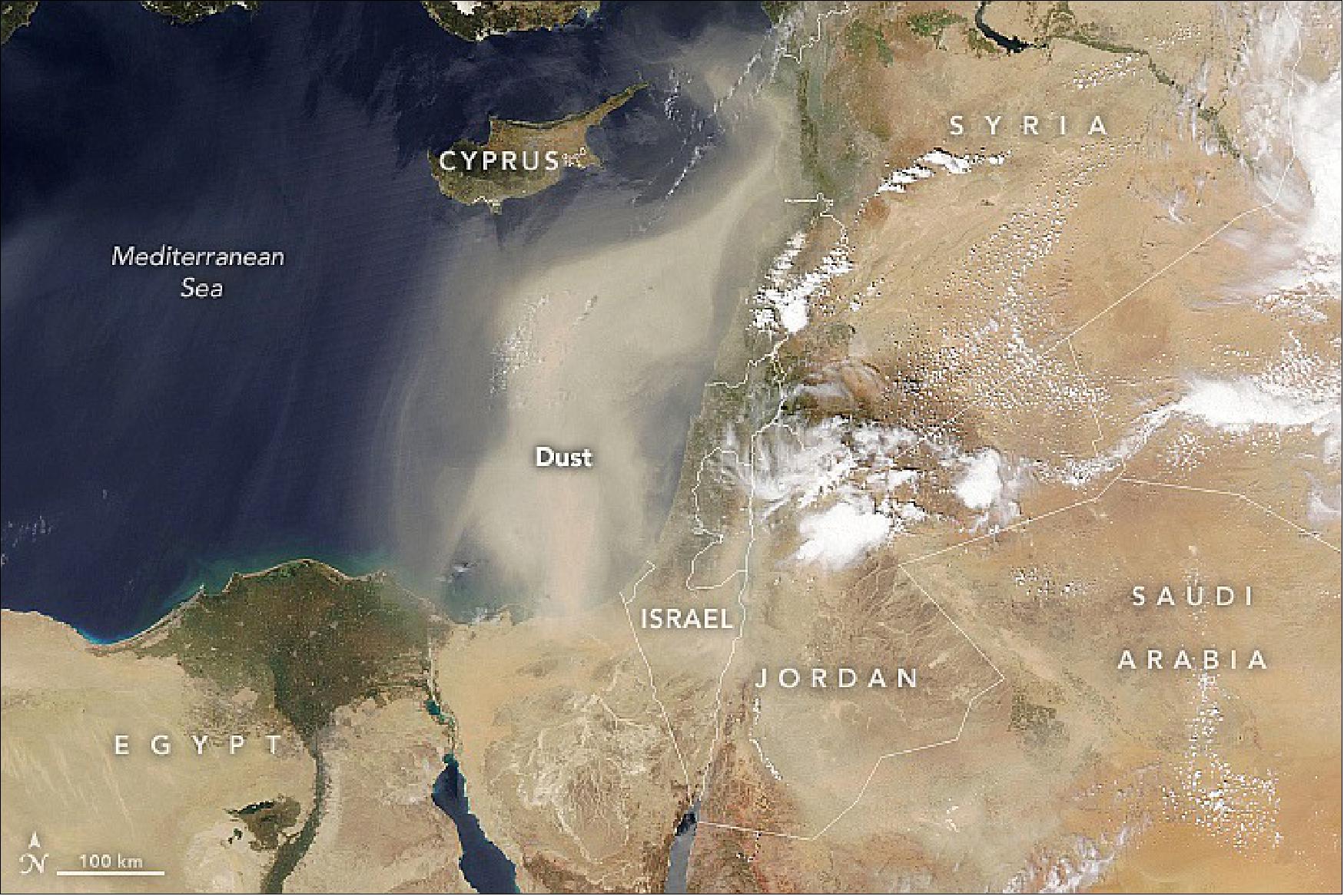
• May 2, 2022: A dust storm over the Middle East in late April 2022 was triggered by thunderstorms that also brought hail and flash floods. The dust turned skies yellow, reduced visibility, disrupted aviation, and degraded air quality. 17)
- In Israel, the Environmental Protection Ministry and Health Ministry warned people with health risks, such as heart and lung ailments, to stay inside. In Jordan, low-visibility conditions caused by gusting winds carrying dust and sand disrupted aviation. Heavy thunder and hail showers and flash flooding also prompted emergency alerts. In Saudi Arabia, large hail and thunderstorms caused flash flooding.
- The storm arose due to an Red Sea depression. Also called a Red Sea low, this weather system brings a hot air mass from the Arabian Peninsula, increasing atmospheric instability that triggers thunderstorms and dust storms, usually during the spring and autumn. In Jordan, most spring dust storms occur in April and form when strong winds blowing over dry, desert soils in eastern and southern Jordan become hotter and drier,
- According to a World Bank report on sand and dust storms, land-use changes in the past few decades have increased the number of dust sources in the Middle East, although most are still largely natural sources like deserts and dry river beds.
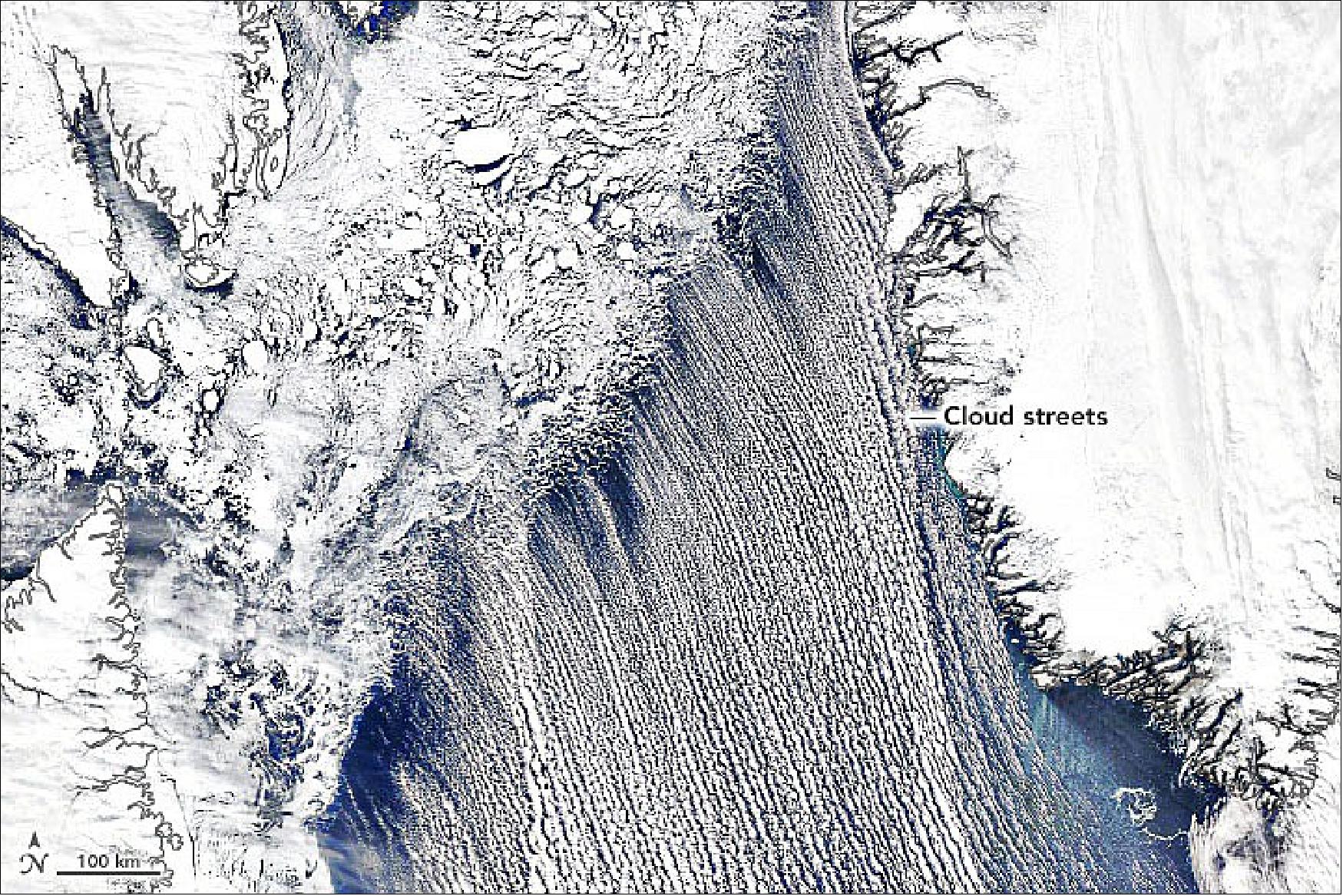
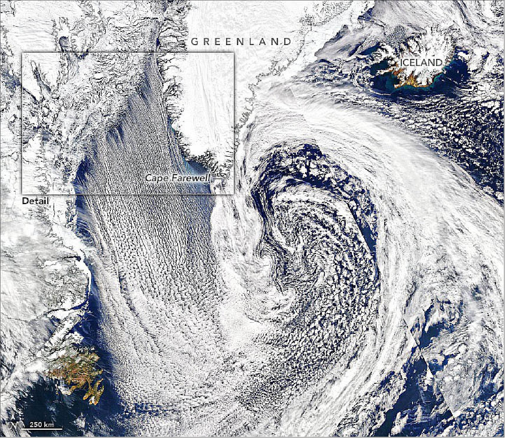
• April 28, 2022: A few times every spring, the skies over the Labrador Sea fill with row after row of long, parallel bands of cumulus clouds. The magnificent organization of these clouds, known as cloud streets, was on full display when this image was acquired on April 19, 2022. 18)
- The appearance of cloud streets indicates that strong, cold winds were blowing toward the southeast over comparatively warmer water. In springtime, sea ice has already entered the melting season, but there is still plenty of ice over land and sea to produce very cold, dry air. There is also enough open water from which that air can draw moisture and form clouds.
- The pattern is the result of the ice-chilled air being warmed by the ocean surface and forming strong currents of upward moving air, or thermals. The moist air rises until it hits a temperature inversion, which acts like a cap and causes the air to roll over and form parallel cylinders of rotating air. On the upper side of these cylinders (the rising air), clouds form. Along the downward side (descending air), skies are clear.
• April 26, 2022: Fire season in New Mexico arrived early and aggressively in 2022, fueled by strong, gusty winds, extremely low humidity, and an exceedingly dry landscape. As of April 19, nearly 99 percent of the state was dealing with some level of drought, according to the U.S. Drought Monitor, with 63 percent rated at extreme to exceptional levels of dryness. Amid those conditions, nearly 137,000 acres of forests and grasslands were burning in five major fires across New Mexico on April 25. 19)
- To the east of Santa Fe, the Hermits Peak fire had consumed 56,478 acres and was 12 percent contained as of April 25. The event began as a prescribed burn in part of the Santa Fe National Forest, but erratic, gusty winds blew it out of control. Strong winds on April 22-23 pushed the fire through steep terrain and caused a merger with the Calf Canyon fire, creating a fire complex with more than 180 miles of perimeter. Residents in parts of San Miguel, Mora, and Colfax counties were told to evacuate their homes.
- To the northeast, the Cooks Peak fire burned through 51,982 acres and was 9 percent contained by the morning of April 25.
- Nearly 1,000 state and federal firefighters were working to contain the Cooks Peak and Hermits Peak blazes, as well as three others across northern New Mexico. According to news reports, hundreds of structures have been burned. Calmer winds and cooler weather on April 24 aided the fire crews, as did some light snow and rain on April 25. But dry and windy conditions are back in the forecast for later this week.
- According to the National Interagency Fire Center on April 25, fourteen large, active fires were burning across 244,000 acres in eleven states. Since the start of 2022, at least 20,262 wildfires have burned 865,290 acres in the United States, well above the 10–year average through April.
- In research published in November 2021, scientists found that burned acreage from wildfires in the western United States doubled between the period of 1984–2000 and 2001–2018. They attributed the increase in fire to a significant change in the vapor pressure deficit, a measurement of how hot and dry the atmosphere can get. Global warming, they noted, has been intensifying vapor pressure deficits, making vegetation more susceptible to burning and the atmosphere more conducive to sustaining fire. Other researchers also found that wildfires have been spreading to higher elevations in the U.S. West in recent decades. 20)
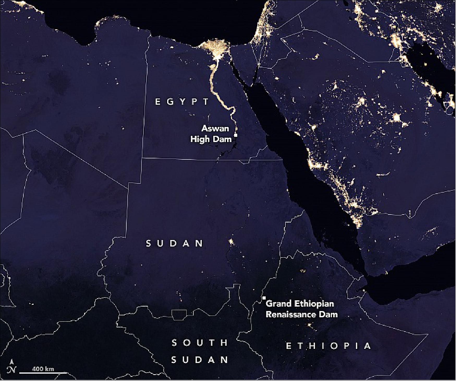
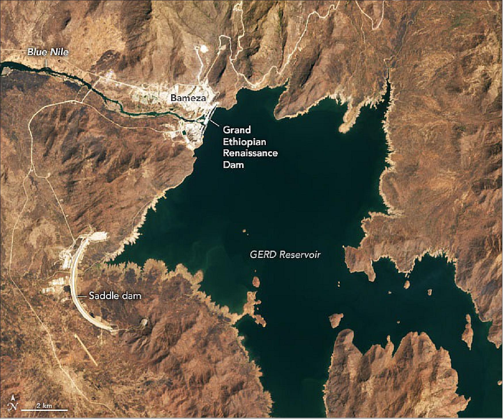
• April 19, 2022: About half of the citizens of Ethiopia have access to electricity, a lower percentage than most other countries in Africa and a much lower percentage than most other countries in the world. To change this, the Ethiopian government began constructing a dam on the Blue Nile in 2011 that will rank as Africa’s largest hydroelectric dam when completed in 2023. 21)
- With three spillways and 13 turbines, the concrete structure will rise 145 meters (475 feet) and create a reservoir that will cover 1,874 km2 (724 square miles) of land, an area about the size of Houston, Texas. Called the Grand Ethiopian Renaissance Dam (GERD), it should more than double Ethiopia’s output of electricity.
- If it works as planned, GERD will usher in a new era and help brighten the mostly dark landscape that appears in nighttime images of Ethiopia. (In the Suomi-NPP satellite image of Figure 28, note the contrast between the darkness of Ethiopia and the bright trail of light along the Nile River in Egypt, where World Bank data indicates that 100 percent of the population has access to electricity.) In addition to generating electricity, GERD should temper destructive seasonal floods in Sudan, boost food supplies in Ethiopia by providing reliable irrigation water, and extend the lifespan of other dams downstream on the Nile by trapping sediment.
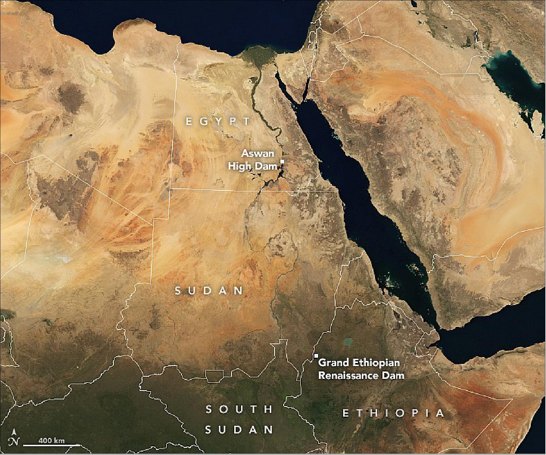
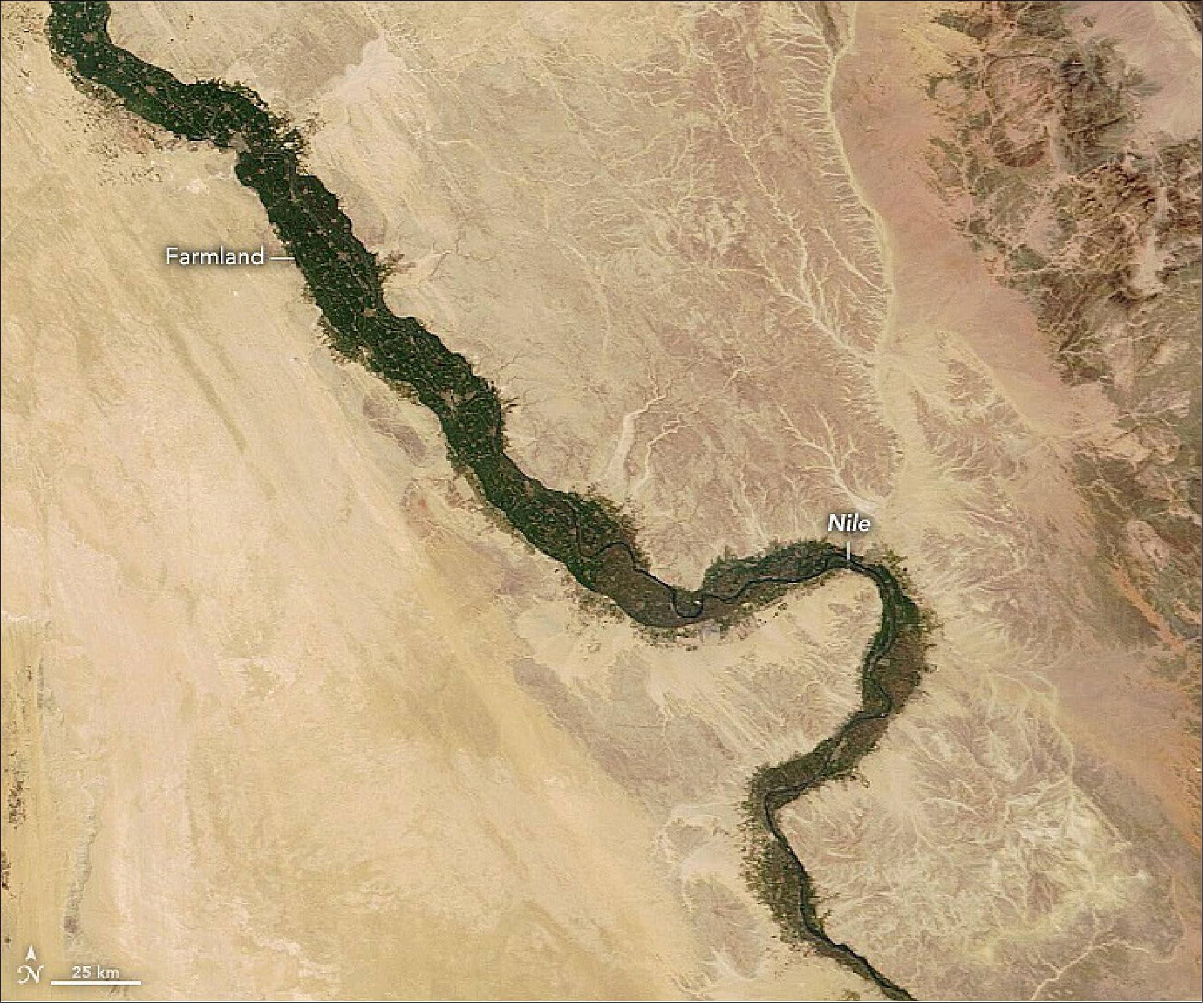
- However, by changing the river’s hydrology, the dam may have an impact on millions of people who live and farm downstream in Egypt and parts of Sudan and use the Nile’s water. The natural-color image of the Nile’s Great Bend shown in Figure 30 underscores how much the people of Egypt depend on the Nile: 95 percent of Egypt’s farmland is found within a narrow zone near the riverbanks.
- After 10 years of construction, GERD is almost complete. In 2020, water managers started filling the reservoir, a process that could take from a few years to a decade depending on weather conditions and how much of the Blue Nile’s flow the dam managers hold back. Ethiopia has an incentive to fill the reservoir quickly to start generating power and start paying for the $5 billion dollar project. However, rapid filling could significantly reduce the water downstream since the Blue Nile provides 60 percent of the water that flows into the Nile.
- “While the dam will certainly have positive effects in regards to flood control and hydroelectric power, there are important unanswered questions about how quickly the reservoir should be filled, and how it will be managed long term,” said Essam Heggy, a NASA Jet Propulsion Laboratory scientist who recently coauthored a study analyzing the potential hydrological and economic consequences of filling the dam at various rates. 22)
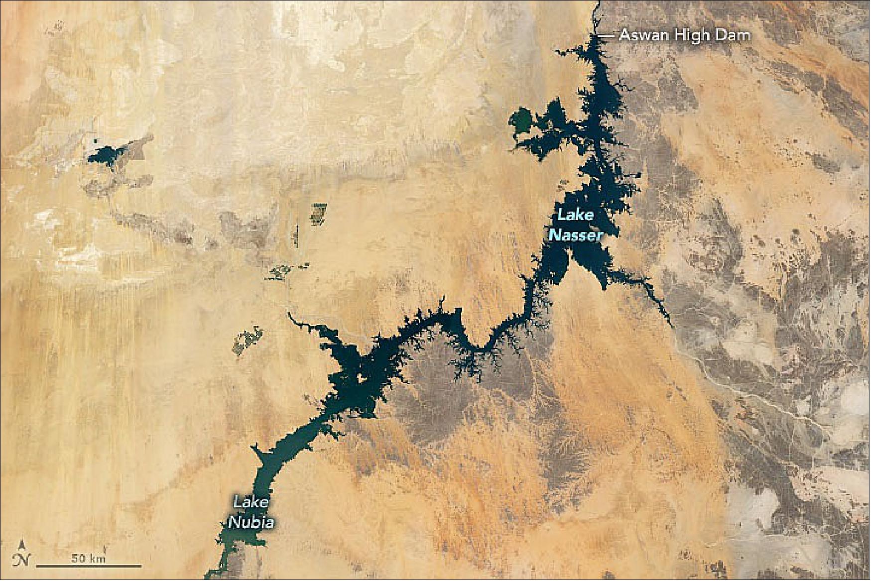
- “Filling the reservoir too quickly—in less than seven years—could lead to measurable water shortages downstream that impact food production, especially if the initial filling occurs under drought conditions,” said Heggy. His research indicates that rapid filling of the reservoir could lead to severe economic losses, though he notes that expanding groundwater extraction, adjusting the operation of Egypt’s Aswan High Dam, and cultivating crops that require less water could help offset some of the impact.
- Egypt, Ethiopia, and Sudan have not agreed on a timetable for filling the reservoir or a plan for how the dam will be managed. Meanwhile, remote sensing scientists have used satellites to help track developments at GERD. Satellites offers one of the best ways to monitor developments because the data are free, transparent, and available to all.
- As of February 2022, one team led by University of Virginia researchers estimated that the GERD reservoir was less than 15 percent full based on satellite observations. “By combining cloud-penetrating radar observations from the European Space Agency’s Sentinel-1 satellite with a NASA digital elevation model of the terrain, we are able to estimate the change of the volume of water in the reservoir,” explained Prakrut Kansara, the lead author of a study published in Remote Sensing that detailed their technique. 23)
- “The reservoir was 23 percent full in September 2021, the end of the rainy season, but then water levels dropped some due to evaporation and water releases,” explained Hesham El-Askary, an earth scientist at Chapman University and one of the study coauthors. “During the first two years, we have seen a filling rate of roughly 11 percent per year, meaning it would take a little less than nine years to be completely full at this rate.”
- The team also used data from NASA’s GRACE and GPM satellites, and results from a NASA model called the global land data assimilation system to analyze the seasonal variability of precipitation, total runoff, and total water storage (which includes surface, subsurface, and groundwater) in the region since 2002.
- “Our research underscores that the Nile Basin experiences dry and wet spells that are linked to the cycles of El Niño and La Niña,” said Venkataraman Lakshmi, another of the study’s coauthors and a professor of engineering at the University of Virginia. “It’s important that we account for these cycles and that they get built into the planning process. We really need to have scientists, engineers, and diplomats in the same room talking to each other about how to go about filling and managing the reservoir.”
- The third filling phase will likely begin in July 2022 and is expected to capture a larger volume of water than the first two fills. “The first filling phase in 2020 impounded about 4.9 billion cubic meters of water and the second phase added another 6 billion cubic meters. If Ethiopia proceeds to fill the GERD in five years, the fourth and fifth fillings could exceed 25 billion cubic meters each,” explained Heggy.
- Whatever the rate of filling, there will be plenty of changes to monitor from both the ground and above in the coming years. “Aswan High Dam and GERD together are capable of retaining more than 280 percent of the Nile’s annual flow,” said Heggy. “The world’s longest river will be mainly driven by the operation of two dams rather than by natural processes.”
• March 22, 2022: High winds, low humidity, and drought-parched grasses fueled a rash of wildfires in Texas, Oklahoma, and Arkansas in mid-March 2022. According to the Texas A&M Forest Service, at least 178 wildfires have burned more than 108,000 acres across Texas in the past seven days, including one of the largest blazes (by area) in state history. At least three first responders have died in Texas and Oklahoma while responding to the fires. 24)
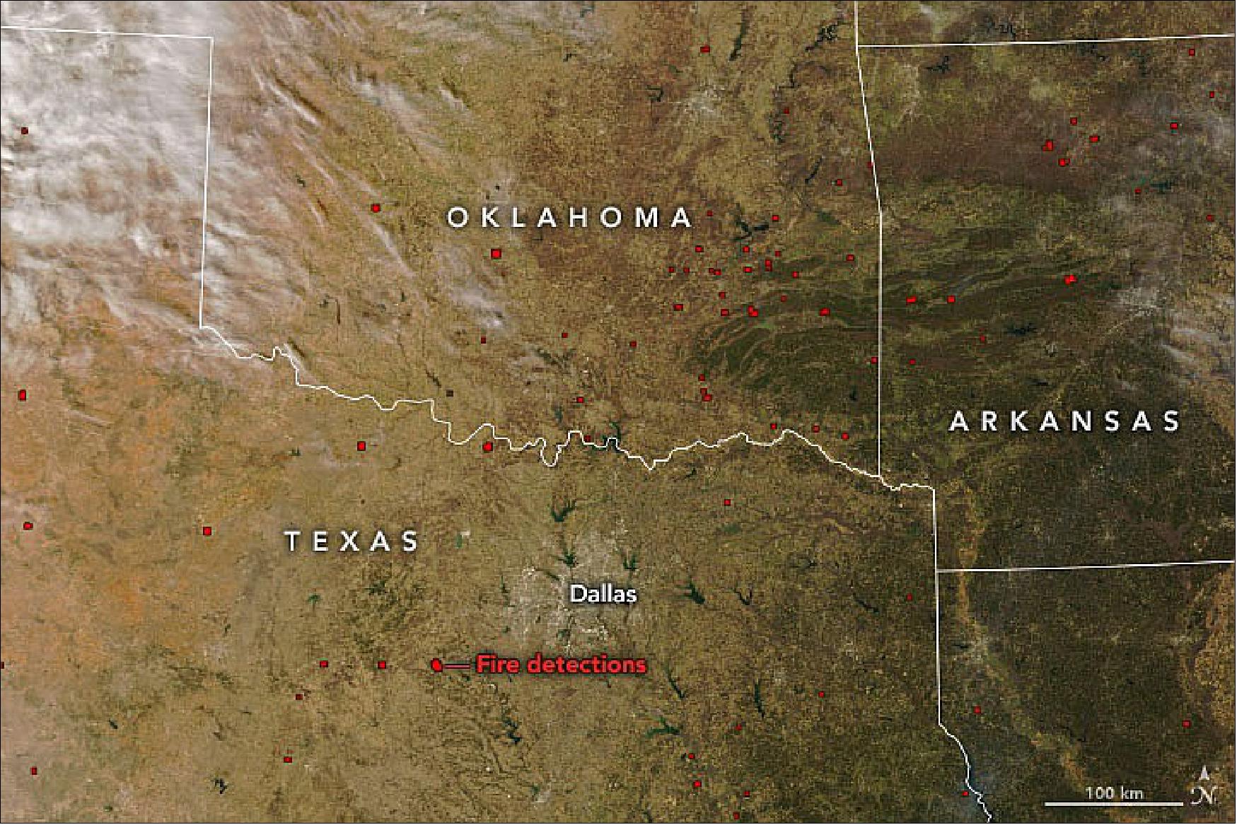
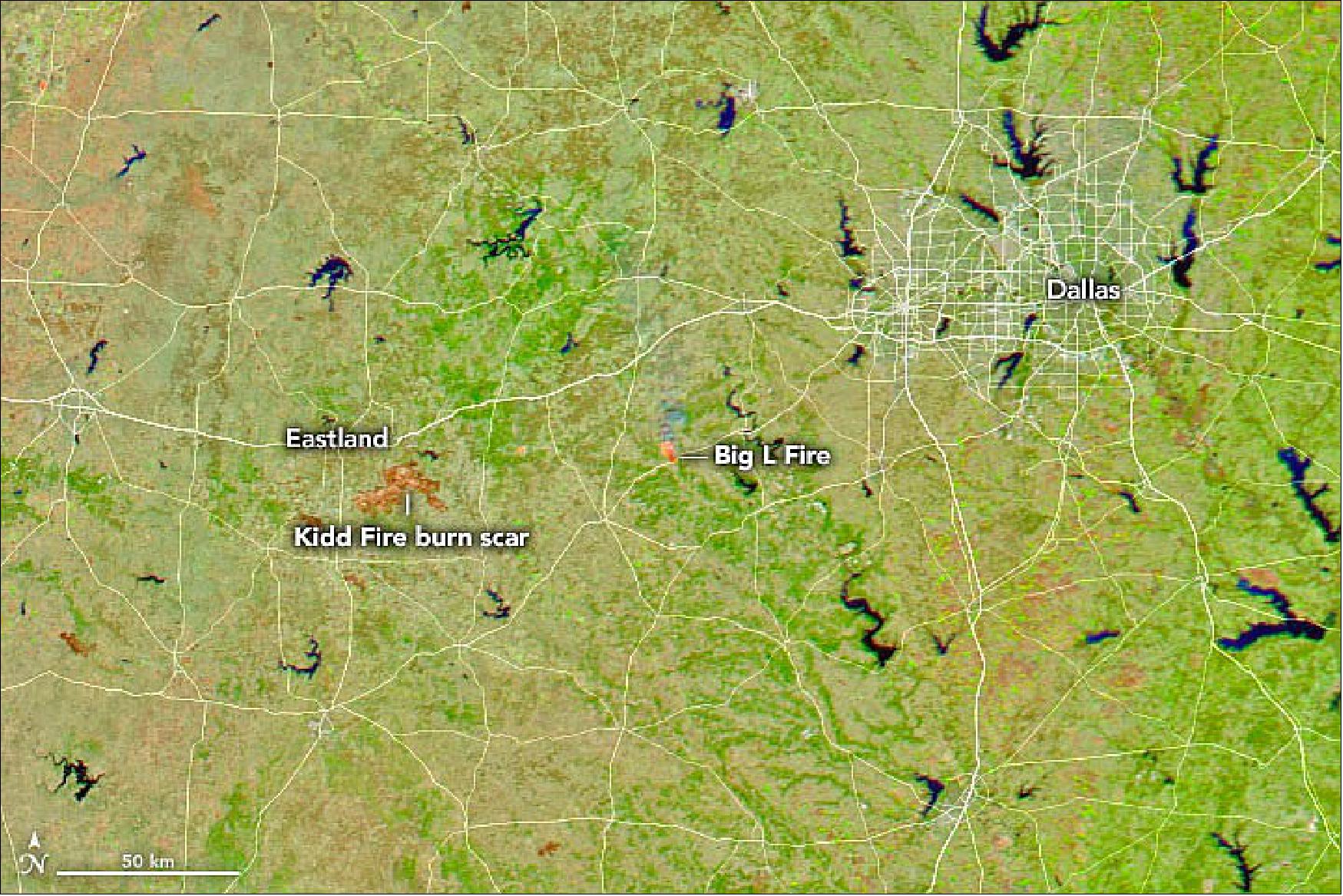
- About 125 miles west of Dallas, the Kidd Fire ignited on March 17 amid days of strong, dry winds. (This short time-lapse sequence shows dust and clouds caught up in the winds.) More than 42,000 acres (65 square miles) have burned so far in a fire that is about 40 percent contained. At least 147 homes and structures have been consumed, including most of the town of Carbon. The Kidd Fire is one of seven that have been grouped into the Eastland Complex by firefighting agencies; more than 54,000 acres (84 square miles) of wildland and property have burned near the town of Eastland.
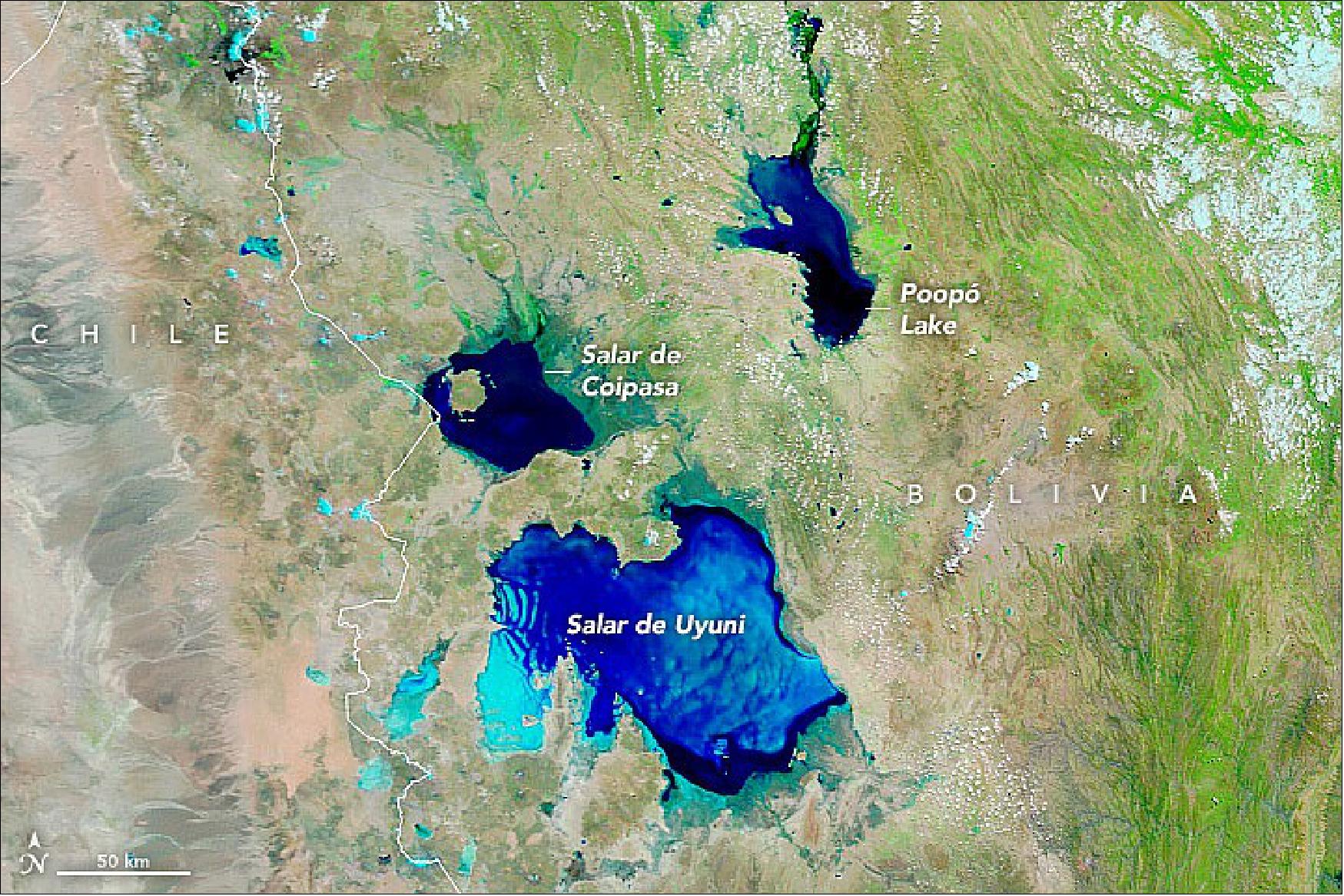
• February 28, 2022: Bolivia’s Salar de Uyuni is the largest salt flat (or playa) in the world. For much of the year, it stretches out in a seemingly endless expanse of white, with a salt crust covering 10,000 km2 (4,000 square miles). During the rainy season, water can fill part of the salt flat and give it a stunning, mirror-like appearance. In early 2022, that watery mirror grew larger and lingered longer than it has in several years. 25)
- Abundant rainfall around the Altiplano in November, December, and early January had the Salar de Uyuni brimming with water nearly to its edges. In fact, local newspapers reported flooding in some areas and temporary prohibitions on travel across the salar during the busy tourist season.
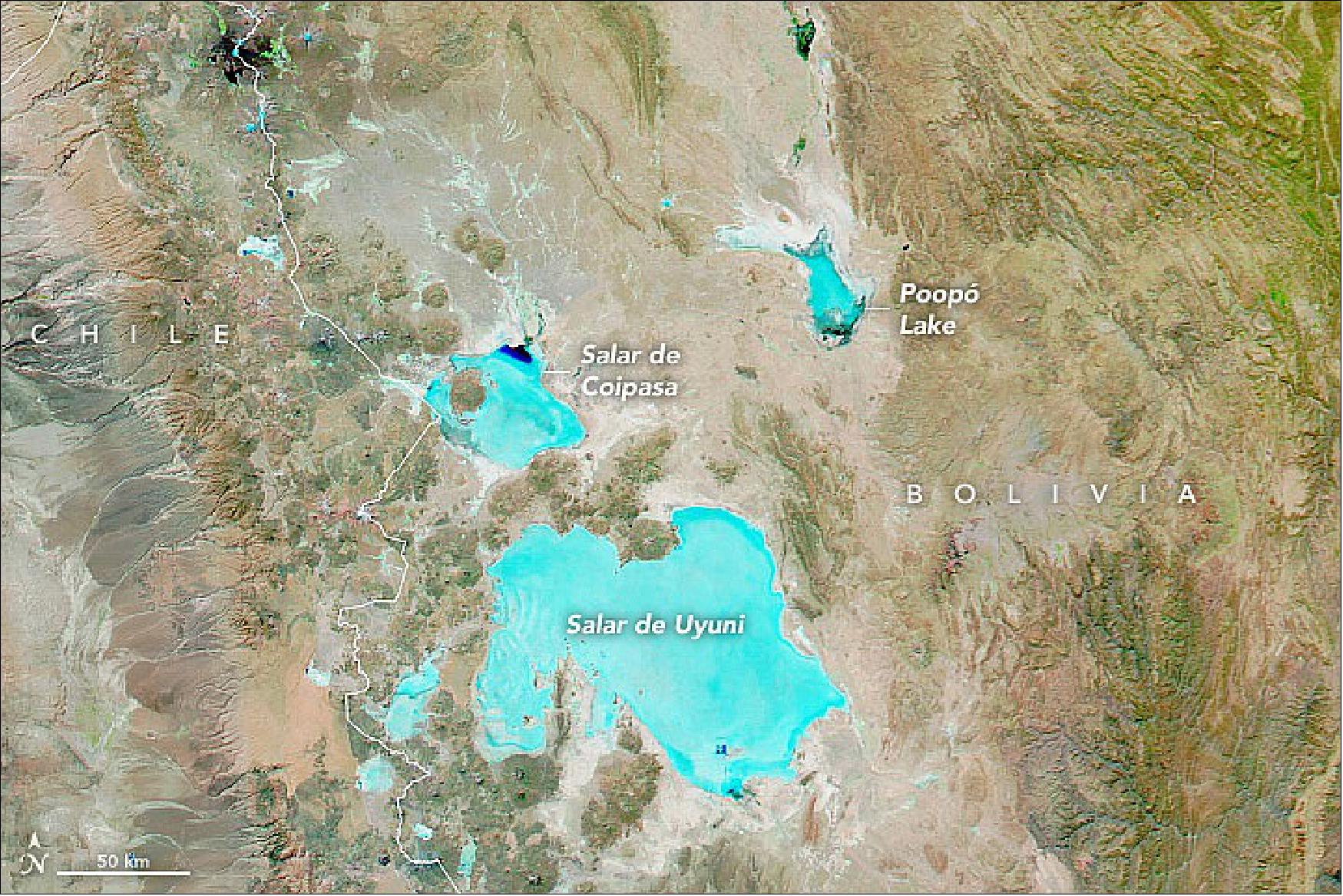
- “The extent of the filling of Salar de Uyuni this year is above normal. The rainy season started earlier than previous years, and rainfall was well above average over the southern Altiplano,” said hydrologist Jorge Molina Carpio of the Universidad Mayor de San Andrés. “This was probably related to the onset of a significant La Niña event. Strong La Niñas during the rainy season are related to positive rainfall anomalies in the southern Altiplano.”
- “Along the Altiplano, but especially in its southwestern edge, precipitation is largely concentrated in austral summer, when transient periods of intense convection are fueled by moisture from the Bolivian lowlands and Amazon basin. The rest of the year is bone dry,” said René Garreaud, a climate scientist at the University of Chile. High-level winds, which vary from season to season and with La Niña and El Niño events, control when and how much moist air rides up onto the plateau. “The stronger and more persistent the easterly wind, the more precipitation you get over the Altiplano.”
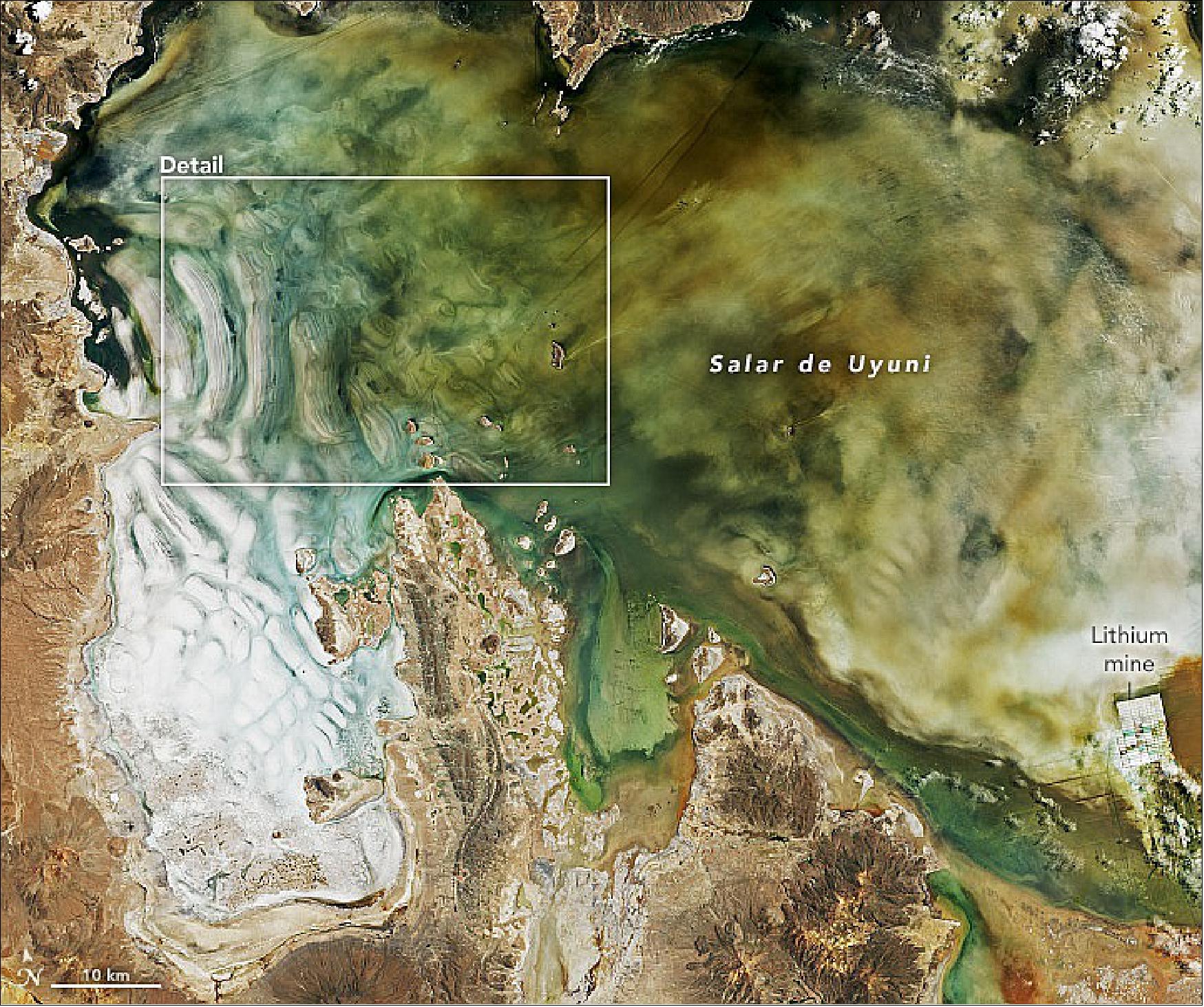
- Garreaud noted that there was a strong easterly flow over the central Andes in December 2021 and early January 2022, leading to abundant rain in the Uyuni-Potosi region. “This area is a closed basin, so all of the precipitation—as rain at the valley floor and snow over the surrounding peaks—contributes to the filling of the Uyuni and Coipasa dry lakes,” he added.
- Salar de Uyuni is rich in minerals—especially lithium (used in batteries), halite (common table salt), and ulexite and gypsum (for fertilizer and plaster)—some of which have been harvested here since at least the 1600s. The stunningly flat landscape draws many tourists who come to see the salty crust in the dry season and the mirror lakes in the wet season. The salt flat is also popular with remote sensing scientists, who use the landscape to calibrate satellite imagers and altimeters.
• February 13, 2022: Tropical Cyclone Batsirai swept over the Indian Ocean and into central and southern Madagascar on February 5–6, 2022, bringing torrential rain, flooding, and high winds. The storm devastated entire villages, killing at least 120 people and leaving tens of thousands displaced, according to the country’s Office of Risks and Disasters. 26)
- The cyclone came just two weeks after the island nation was struck by Tropical Storm Ana, which followed a series of heavy rainstorms in mid-January. Flooding and landslides killed at least 58 people and displaced more than 70,000.
- Batsirai made landfall on February 5 on the southeast coast near Mananjary as a category 3 storm with sustained winds of 165 km (105 miles) per hour and gusts up to 230 km (145 miles) per hour. Heavy rain continued to fall on February 7–8 as the storm moved over the island and off to the southwest.
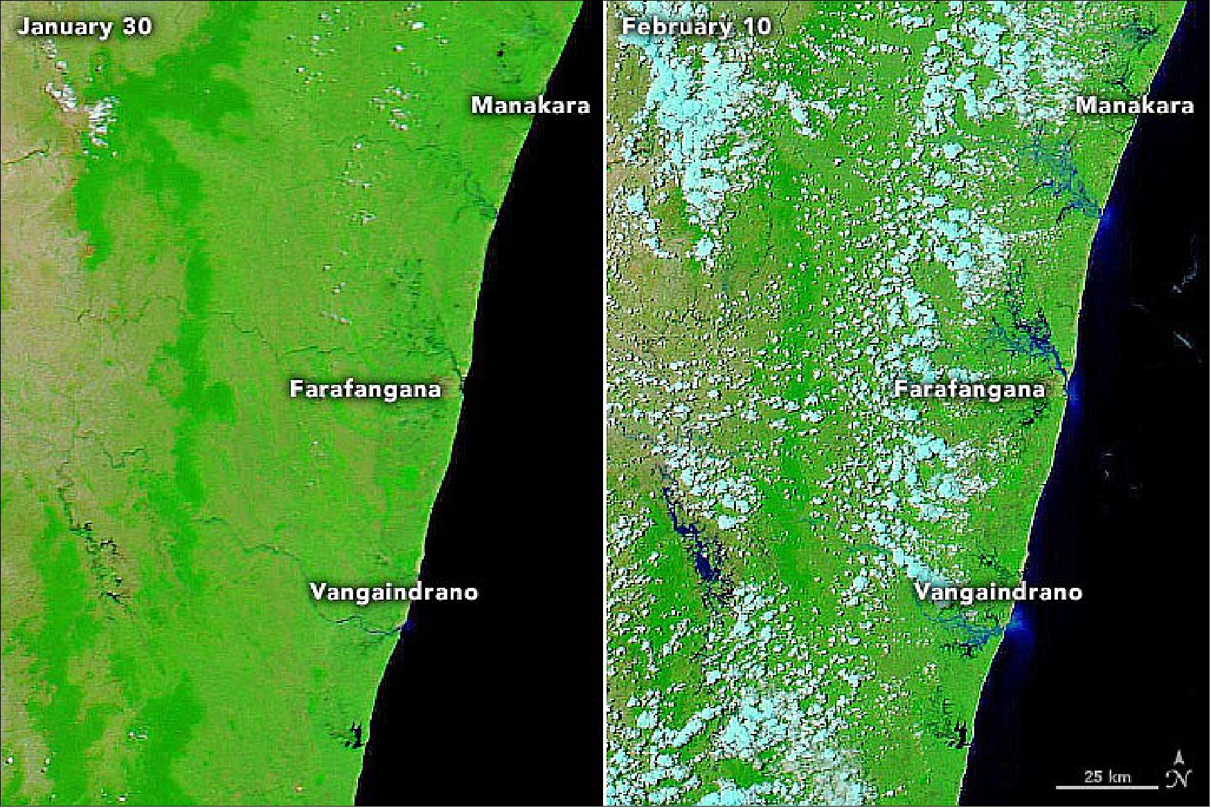
- In its wake, Batsirai left water and power outages, along with destroyed or damaged buildings and schools. Relief efforts were underway, although washed out roads and bridges have made some areas inaccessible, according to the United Nations Office for the Coordination of Humanitarian Affairs.
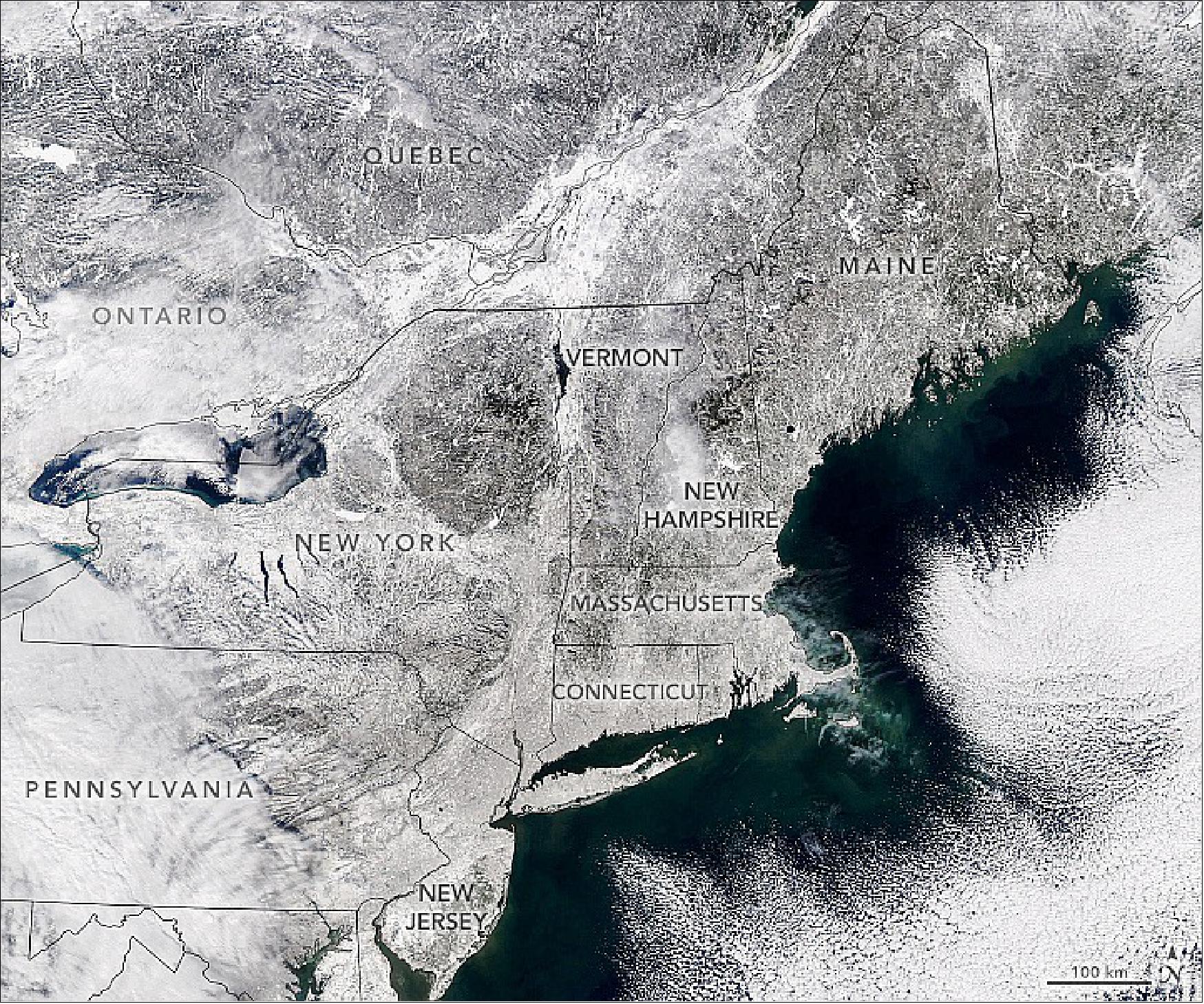
• February 1, 2022: After several mostly uneventful months of winter, the densely populated northeastern United States was buried in mounds of snow and blasted by gale-force winds on January 28-29, 2022. Twelve states from North Carolina to Maine received measurable snowfall from the nor’easter; eight of them had towns report more than a foot (30 cm) of snow. 27)
- Due to the moderating effect of warmth and moisture from the ocean, coastal areas often see less snow during winter storms. But in this case, the New Jersey shore, Long Island, and coastal New England from New London to Cape Cod to Boston drew the greatest snowfalls, with some areas seeing the flakes fly at rates up to 3 to 4 inches per hour. According to National Weather Service (NWS) reports, more than 21 inches of snow were measured in Providence, Rhode Island; 29 inches fell in Norton, Massachusetts, 30 in Quincy; and 22 inches dropped on Norwich, Connecticut. Boston tied a record for the most snowfall in a 24-hour period with 23.6 inches, and Islip, New York, had its second-highest daily total (23.2 inches).
- The potent nor’easter also brought strong winds sometimes approaching hurricane force. The NWS determined that blizzard conditions were reached in multiple locations in Rhode Island and Massachusetts, affecting as many as 11 million people. A blizzard is defined as a period of at least three hours with falling snow, persistent wind gusts above 35 miles (55 kilometers) per hour, and visibility below 0.25 miles (0.4 kilometers). Marshfield, Massachusetts, endured such conditions for 12 hours, Newport for 9.5, and Boston for 7.5. Wind gusts reached the strength of a category 1 hurricane on Cape Cod, Cape Ann, and Nantucket.
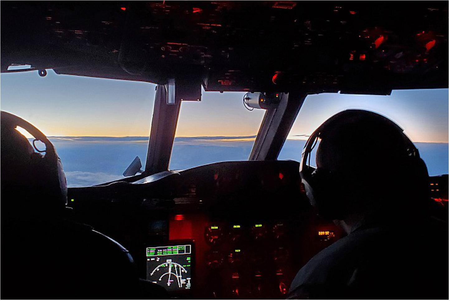
- “Snowstorms are really complicated storms, and we need every piece of data—models, aircraft instruments, meteorological soundings—to really figure out what’s going on within these storms,” said Gerry Heymsfield, a deputy principal investigator for IMPACTS and a scientist at NASA’s Goddard Space Flight Center.
- In recent winters, the team has been tracking rain and snow storms across the Midwest and Eastern United States in two NASA planes equipped with scientific instruments. With a high-altitude ER-2 flying above storms and the P-3 flying within the clouds, scientists have been collecting data about snow particles and the conditions in which they form. Scientists have also been measuring cloud properties from below using ground-based radars.
- Storms often form narrow structures called snow bands, said Lynn McMurdie, principal investigator for IMPACTS and an atmospheric scientist at the University of Washington. One of the main goals is to understand how these structures form, why some storms do not have snow bands, and how snow bands can be used to predict snowfall.
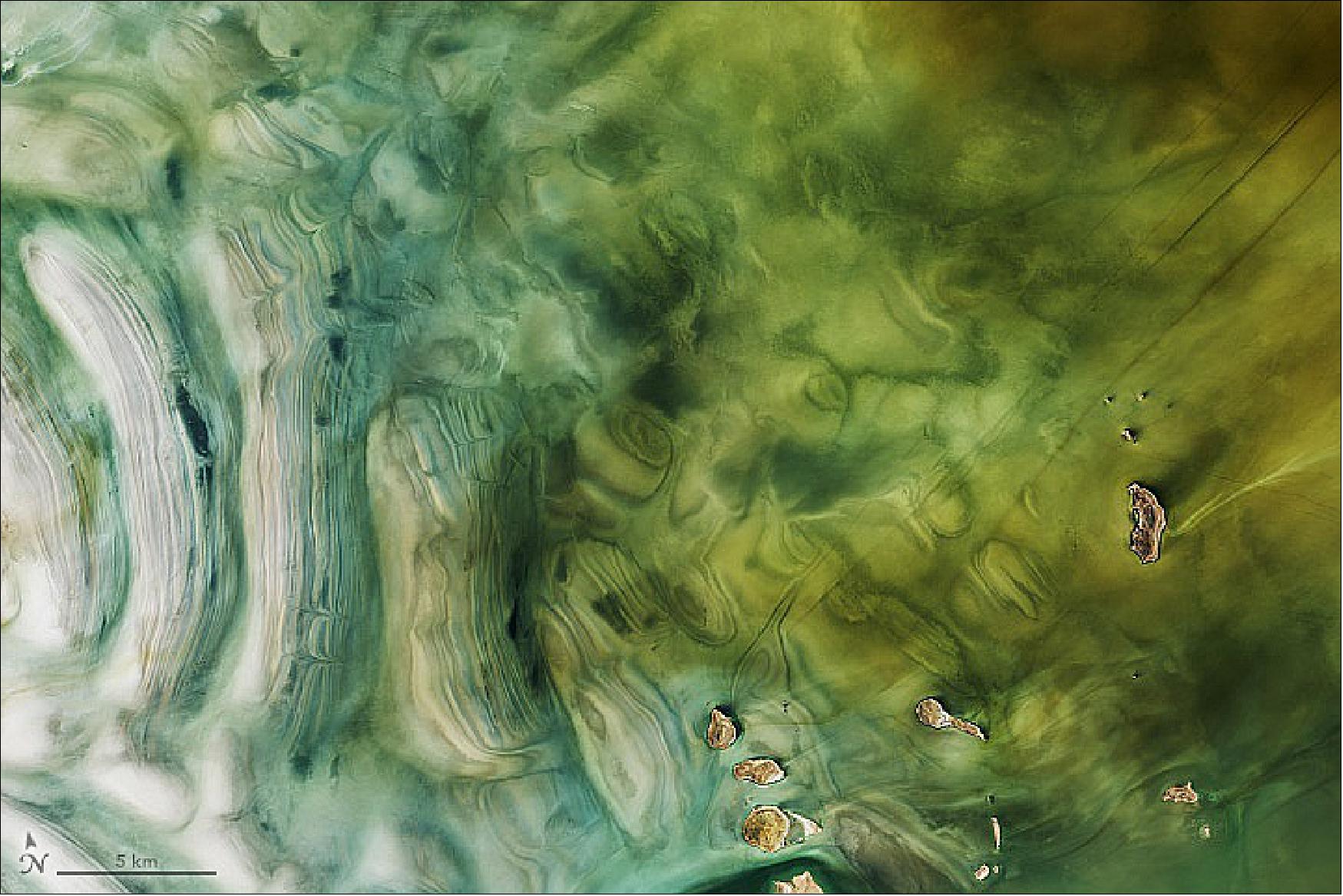
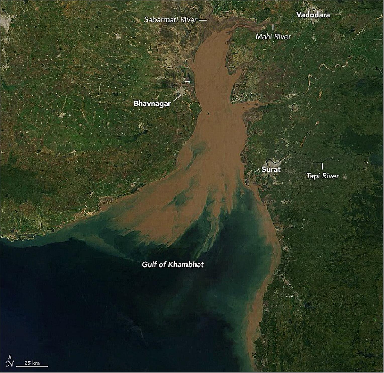
• January 29, 2022: The Gulf of Khambhat lies on the west coast of India between the Saurashtra Peninsula and mainland Gujarat. Several major river systems—including the Narmada, Tapi, Mahi, Sabarmati, and Shetrunji—deliver abundant freshwater and heavy sediment loads to the gulf. The gulf measures 80 km (50 miles) wide at its mouth in the Arabian Sea but narrows to about 25 km (15 miles) at its head, where the deltas of the Sabarmati and Mahi rivers meet. 28)
- These natural-color images, acquired by the MODIS instrument on NASA’s Aqua satellite on April 16 and October 16, 2021, show the sediment discharge concentrated at the northern end of the gulf. The monsoon season extends from June to September, leading to increased sediment discharge that is evident in the October image. As freshwater begins to disperse and sink at the outer reaches of the gulf, the reflectivity of the sediment changes, appearing green instead of brown.
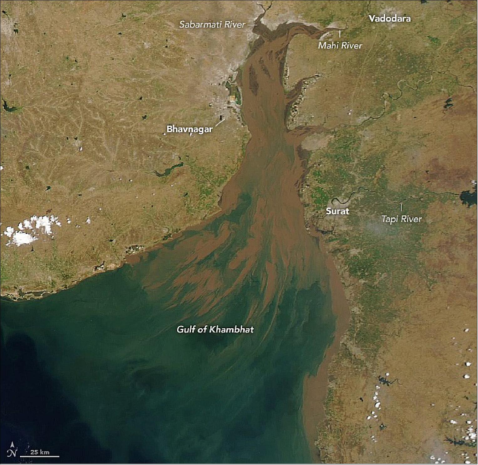
- The currents in the gulf are dominated by these strong tides, which can flow at 1.5 to 2 m/s (3.3 to 4.5 miles per hour). Additionally, the water is less than 20 meters (65 feet) deep in most parts, and receding tides expose vast intertidal areas up to 5 km (3 miles) wide. Extensive mudflats, along with large shoals and banks (see the April image of Figure 43) can make navigation potentially hazardous for even small vessels.
- With all of the dynamic flows in the gulf, the bathymetry (bottom topography) can shift rapidly and pose additional hazards to navigation. This has prompted some researchers to develop a bathymetry model based on satellite radar data. Such a model could allow more rapid updating of charts of bottom features.
• January 15, 2022: For much of 2021, drought gripped southern Iran, parching crops, drying wells, and fueling protests over water. The first week of 2022 brought the opposite problem—a series of potent rain and snow storms overwhelmed rivers and unleashed widespread flooding. 29)
- News and social media reports showed destructive flood waters that washed out bridges, swept away cars, swamped homes, and inundated farmland. The floods have killed at least 10 people and damaged hundreds of homes and vehicles, according to the Iranian Red Crescent Society.
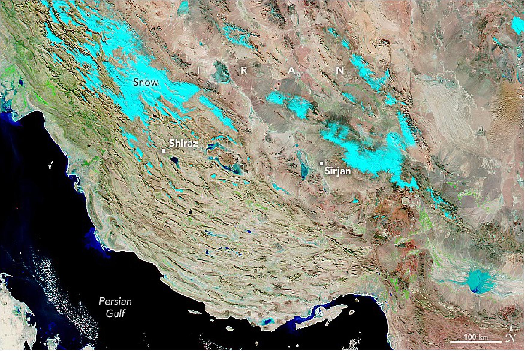
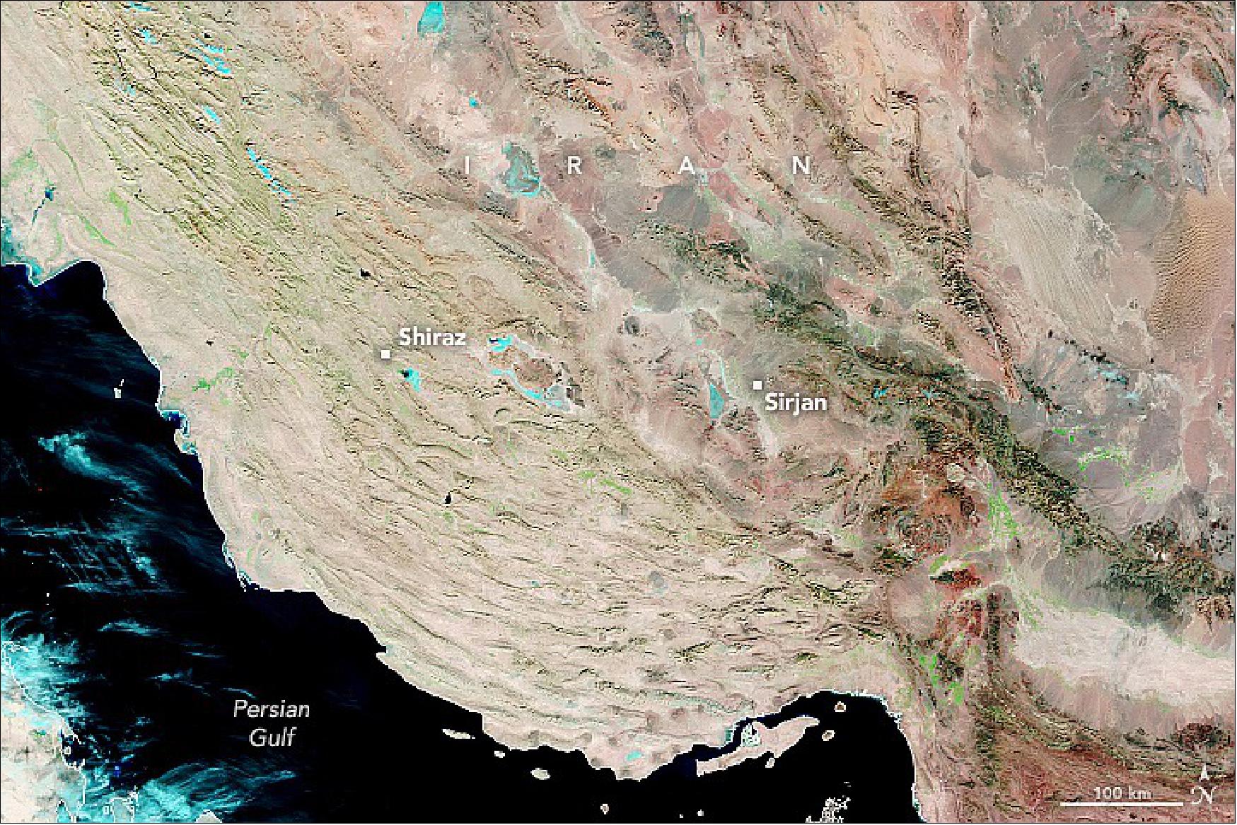
- The recent burst of rain will not necessarily end Iran’s drought or water challenges immediately. While storms can replenish moisture on the surface, it takes a sustained period of wet weather to replenish groundwater, which many people in this region rely on for irrigation. Data collected by the Gravity Recovery and Climate Experiment Follow-On (GRACE-FO) satellites show that reserves of shallow groundwater in the region’s aquifers, though improved, were still low in some parts of southern Iran on January 10, 2021, according to GRACE-FO data published by the University of Nebraska.
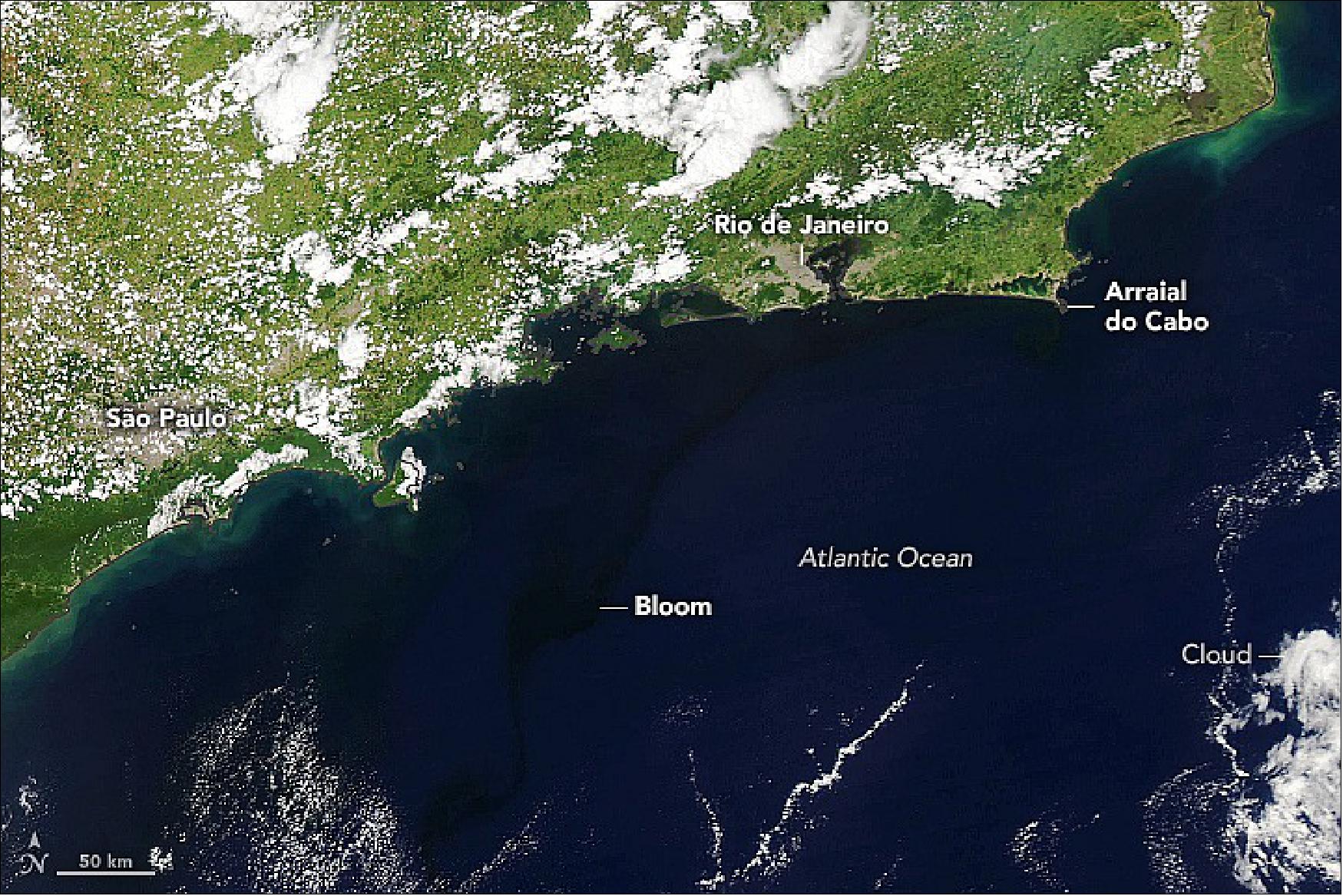
• January 13, 2022: Beachgoers in the Brazilian state of Rio de Janeiro contended in late 2021 with unwelcome ocean-dwelling visitors. Starting in November, countless microscopic phytoplankton amassed along the coast, coloring the clear, blue waters a dark, reddish-brown. The bloom—known as a red tide or harmful algal bloom (HAB) event—was unusually widespread and long-lived. 30)
- Phytoplankton blooms are common this time of year in Rio, but they typically contain species that are beneficial to the ecosystem. In contrast, harmful algal blooms can show up any time of year, usually spurred by sewage effluents and heat waves; they tend to be small and last no longer than a few days. This red tide event spanned more than 200 km of the coastline and lasted more than eight weeks. “It is very worrying,” said Priscila Lange of the Department of Meteorology, Federal University of Rio de Janeiro.
- Some species in a red tide can produce toxins but, so far, those species have not been observed in the Rio bloom. Instead, Lange called the bloom “worrying” because of its likely impact on the marine food web.
- From September to January of most years (spring and summer in South America), cool, nutrient-rich water wells up from the depths of the ocean off Arraial do Cabo, replacing surface waters that have been pushed offshore by winds and the Coriolis effect. The abundance of nutrients and sunlight at the ocean surface triggers blooms of diatoms and other phytoplankton, which are soon consumed by zooplankton and fish larvae. Marine currents push the upwelled water masses west toward the city of Rio de Janeiro, and the warm, blue water off Rio usually turns cold and dark green.
- Spring 2021 was unlike most years. Lange and colleagues think six weeks of cloudiness and rain hampered the usual growth of diatoms and small flagellates, leaving the waters off Rio transparent and brimming with nutrients. When the skies finally cleared in early November, ample sunlight and low turbulence set the stage for the red tide. “Once there was light, the red folks—dinoflagellates, Mesodinium rubrum, etc.—bloomed like crazy!” Lange said.
- The change happened fast. The first visual observations of red tide were made on November 3, then confirmed by water samples taken from a beach in Rio on November 16. The water off Rio’s beaches quickly became very dark, and red seafoam built up.
- In early December, the red tide reached Arraial do Cabo and “darkened the waters of Rio’s most pristine scuba dive paradise,” Lange said. Satellite images from December 5 show the red-brown water spanning the length of the coastline between the two cities.
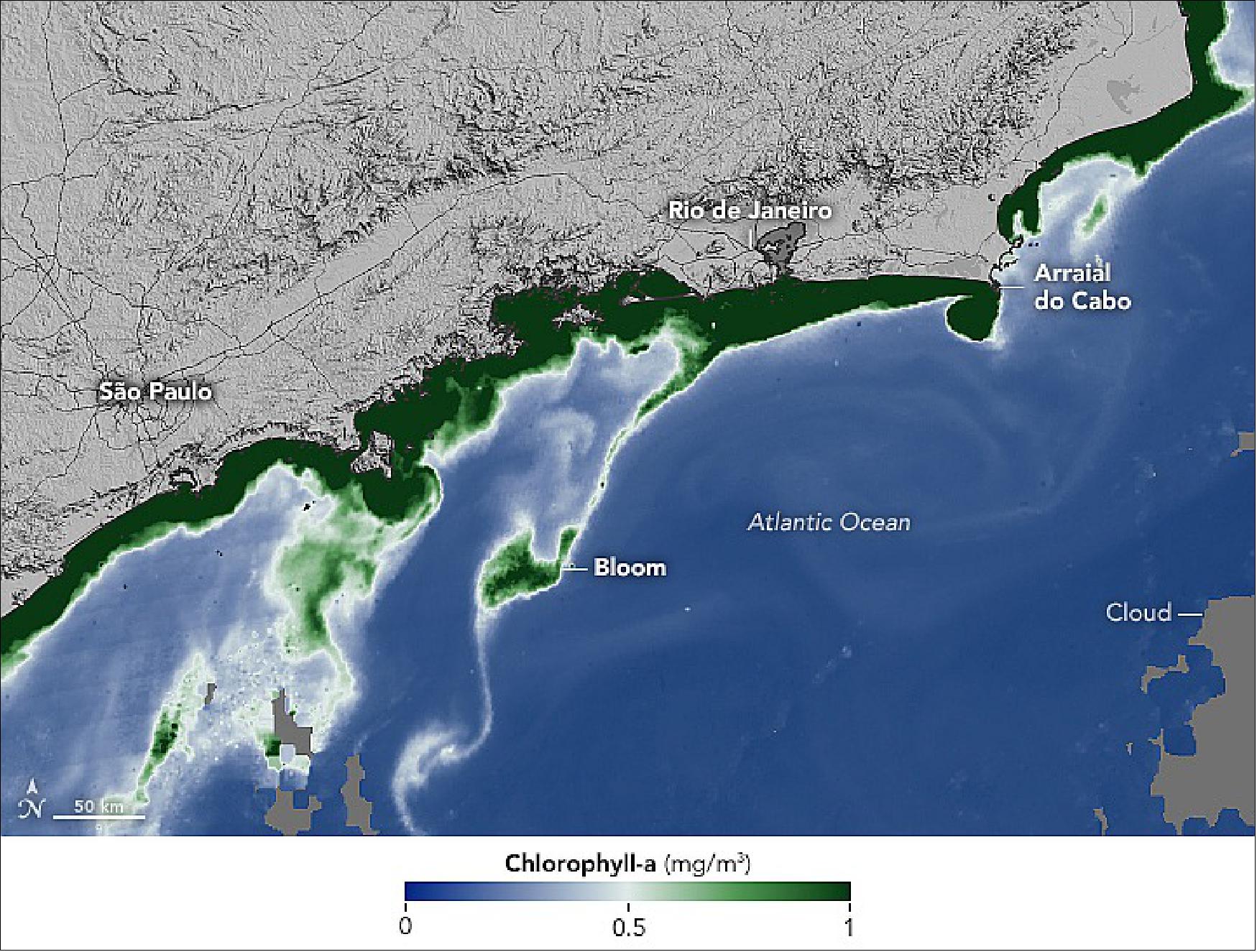
- Lange and colleagues will continue to observe how the bloom progresses. But even after a massive bloom fades, the effects can be lasting. After the phytoplankton die, the process of decomposition by bacteria can deplete the water of oxygen (hypoxia) and cause fish kills. Also, the red tide species can replace other phytoplankton species that usually support a region’s fish and marine food webs.
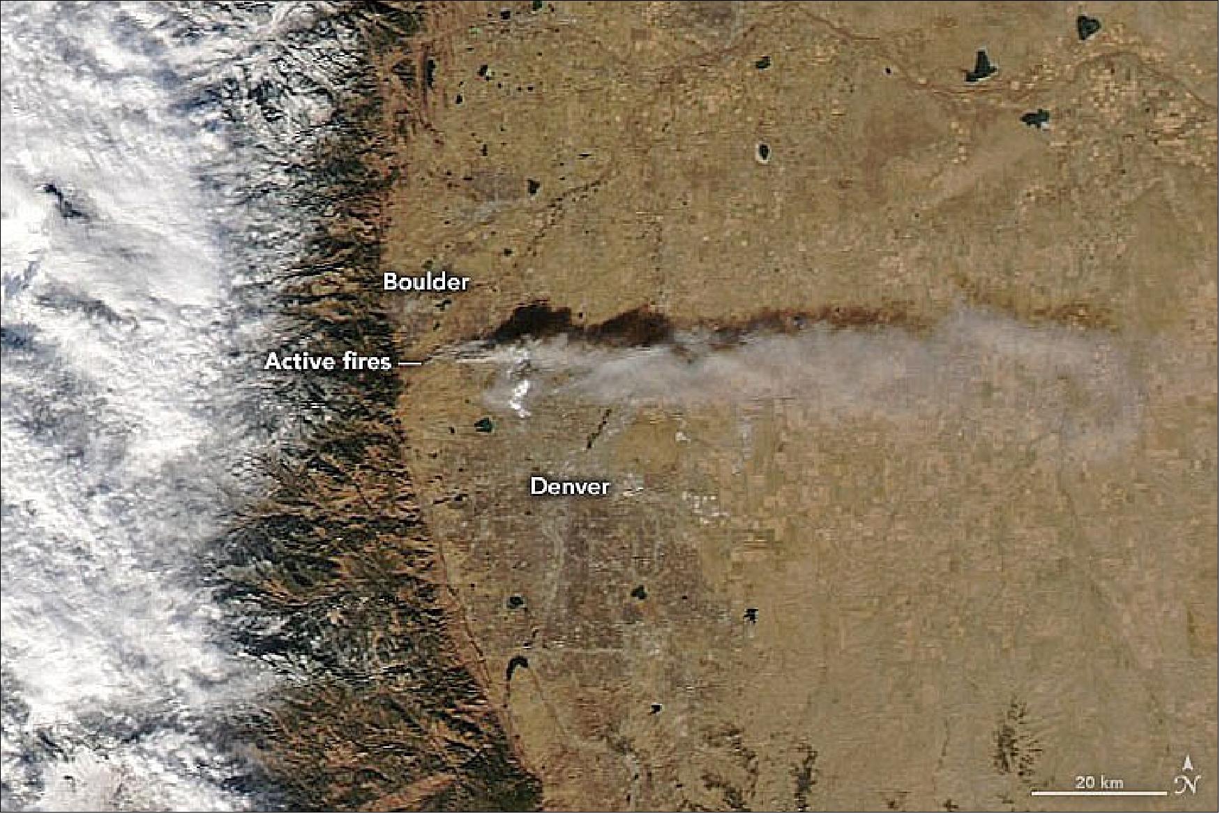
• January 5, 2022: On December 30, 2021, high winds roared out of the west and down the front slope of the Rocky Mountains in Colorado. Northwest of Denver, peak gusts reached 115 miles (185 kilometers) per hour—the equivalent of a category 3 hurricane. Those winds whipped up intense grass and brush fires in south Boulder and blew them east toward the towns of Superior and Louisville, igniting a firestorm. By the time it was over, nearly 1,100 houses had been destroyed or damaged, two people were reported missing, and thousands were displaced. 31)
- The Marshall fire is now the most destructive in the state’s history. Four of the top five largest wildfires on record in Colorado occurred between 2018 and 2021.
- Unlike many of the megafires in the American West in recent years—which typically occur in forests and wildlands—the Marshall fire quickly travelled into densely populated neighborhoods and transitioned from a wildfire to an urban conflagration.
- Tens of thousands of residents were evacuated as flames were blown down streets and through cul-de-sacs. The fire was carried by what climate scientist and Boulder resident Daniel Swain called “an ember storm.” Blown by hurricane-force winds, the embers leapt from house to house, burning many from the inside out, while torching trees, igniting commercial buildings, and jumping a highway.
- The next day brought much-needed moisture, as a cold front moved in and dropped more than 10 inches (25 cm) of snow—dampening the fire but also complicating the response. As of January 3, 2022, the perimeter of the 6,200-acre fire was fully contained.
- High winds and wildfires are not uncommon on the Front Range, but a December wildfire is; the normal fire season lasts from May to September. One recent study found that increases in extreme fire weather are being driven by decreases in atmospheric humidity and increasing temperatures.
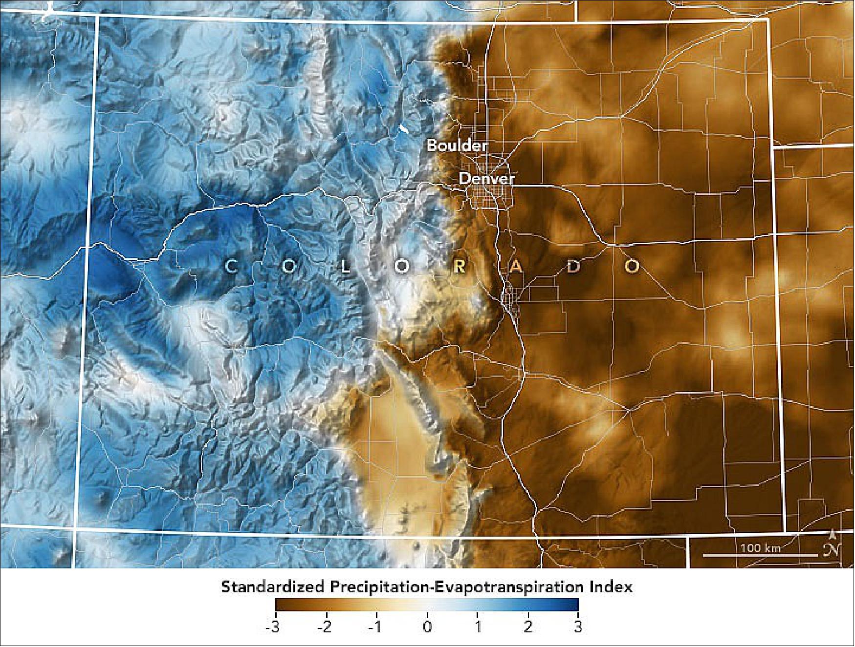
- At the time of the fire, the eastern part of Boulder County was classified with extreme drought, according to the U.S. Drought Monitor. The map above shows the Standardized Precipitation-Evapotranspiration Index (SPEI) for Colorado for the month of December 2021. It accounts for both precipitation and temperature. (It does not include the New Year’s snowfall that helped extinguish the fire.) According to the Colorado Climate Center, SPEI values exceeding minus 2 are very rare and are indicative of the extreme warm and dry conditions across eastern Colorado.
- The map also shows the contrast between the extreme drought in the eastern part of the state, where the fire occurred, and the snowpack in the western part of the state, where significant December snowfalls brought the snowpack near or above average. Denver, which normally has 30 inches of snow by late December, did not record its first winter snowfall until December 10, the latest on record.
Sensor Complement
Aqua has six Earth-observing instruments on board, collecting a variety of global data sets. 32)
Note: The descriptions of CERES and MODIS can be found under Terra.
Instrument | Sponsor | Developer | Spectral resolution | Geophysical parameters |
AIRS | NASA/JPL | BAE Systems | More than 2,300 spectral channels ranging from 0.4 µm to 15.4 µm | Atmospheric temperature and humidity, land and sea surface temperatures, cloud, radioactive energy flux |
AMSR-E | JAXA | JAXA (Japan) | 12 channels at six discrete frequencies from 6.9 GHz to 89 GHz | Precipitation rate, water vapor, surface moisture content, sea ice extent, snow extent |
AMSU | NASA/GSFC | Aerojet | 15 channels ranging from 50 GHz to 90 GHz | Atmospheric temperature and humidity |
HSB | INPE | MMS, UK | Five channels ranging from 150 MHz to 183 MHz | Atmospheric humidity |
CERES | NASA/LaRC | TRW | Cross-track and azimuthal scanners with three channels per scanner | Radiative energy flux |
MODIS | NASA/GSFC | Raytheon (SBRS) | 36 channels ranging from 0.4 µm to 14 µm | Cloud, radioactive energy flux, aerosols, land cover and land use change, vegetation dynamics, land surface temperature, sea surface temperature, ocean color, snow cover, atmospheric temperature and humidity, sea ice |
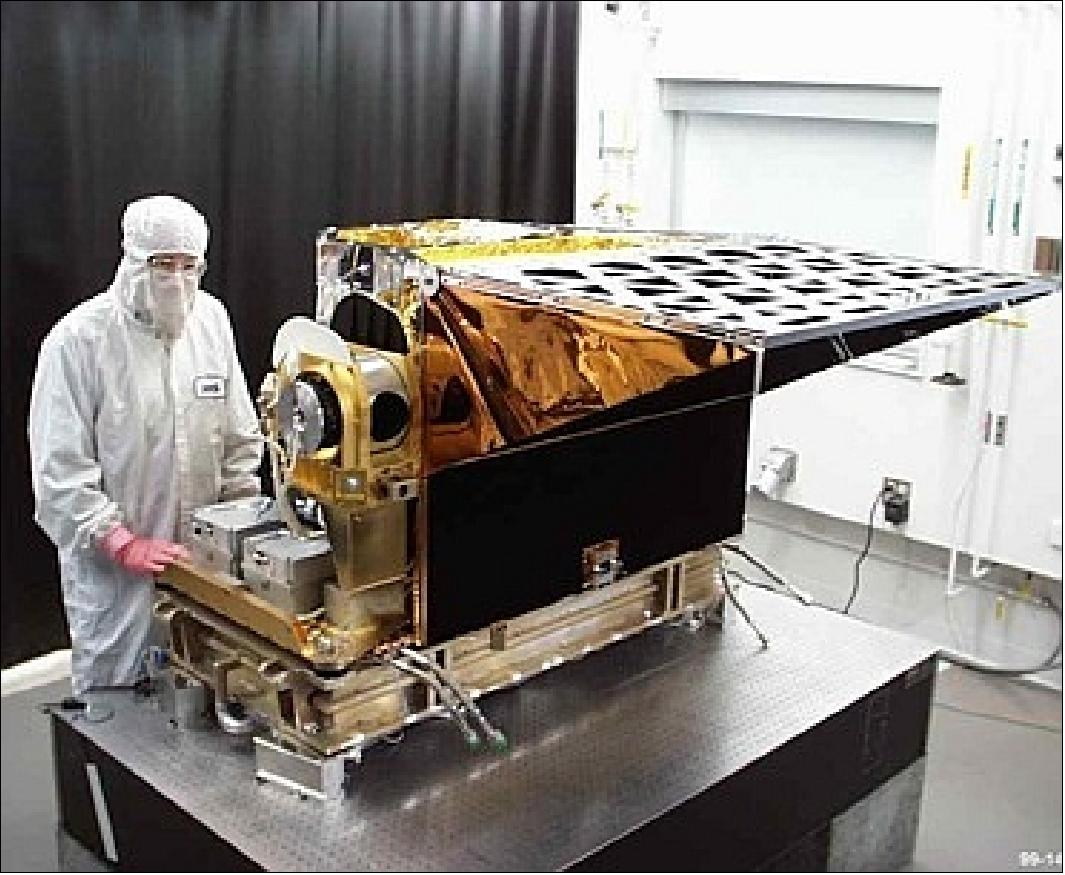
AIRS (Atmospheric Infrared Sounder)
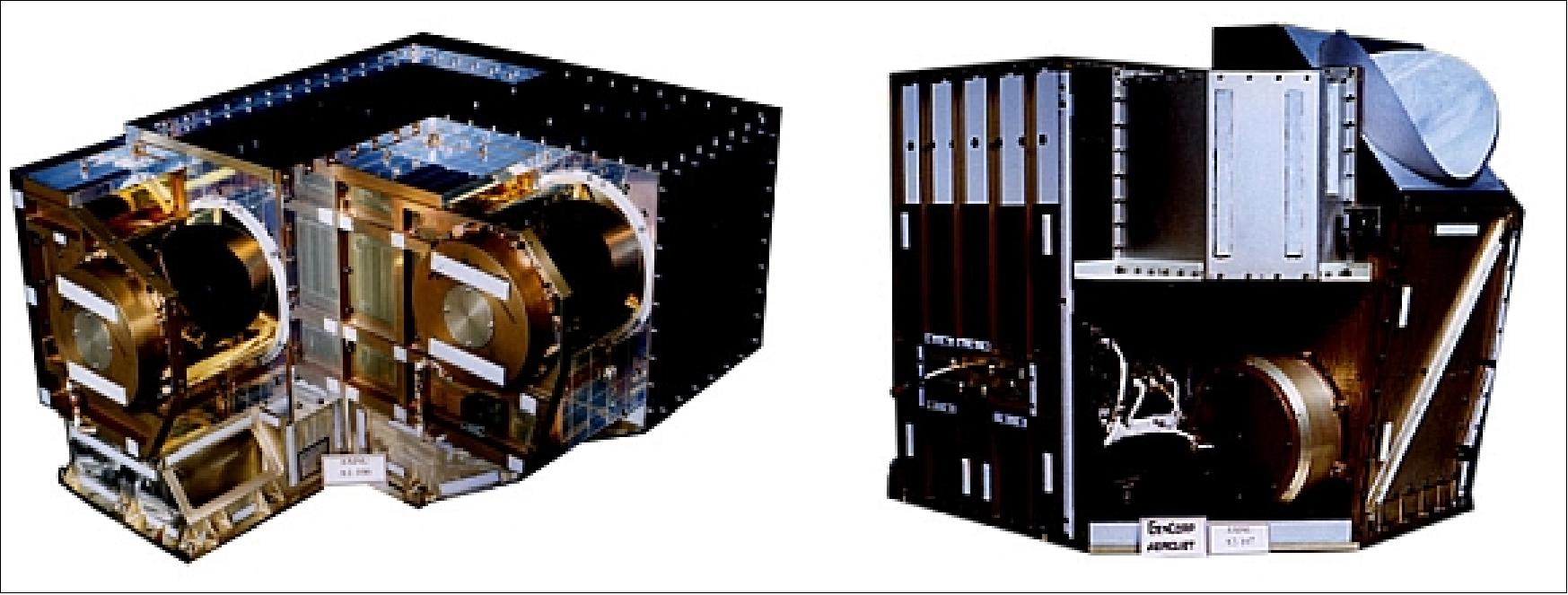
AIRS is a NASA/JPL instrument, PI: M. T. Chahine; prime contractor is BAE Systems (Infrared and Imaging Systems Division (LMIRIS) of BAE Systems, in Lexington, MA). AIRS, along with AMSU and HSB, is of HIRS and MSU heritage flown on the NOAA POES series. Objective: High-spectral-resolution measurement of global temperature/humidity profiles in the atmosphere in support of operational weather forecasting by NOAA. Measurement of the Earth's upwelling infrared radiances in the spectral range of 3.74 - 15.4 µm, simultaneously at 2378 frequencies (bands). Four visible wavelength channels are also present. 33) 34) 35) 36) 37) 38) 39)
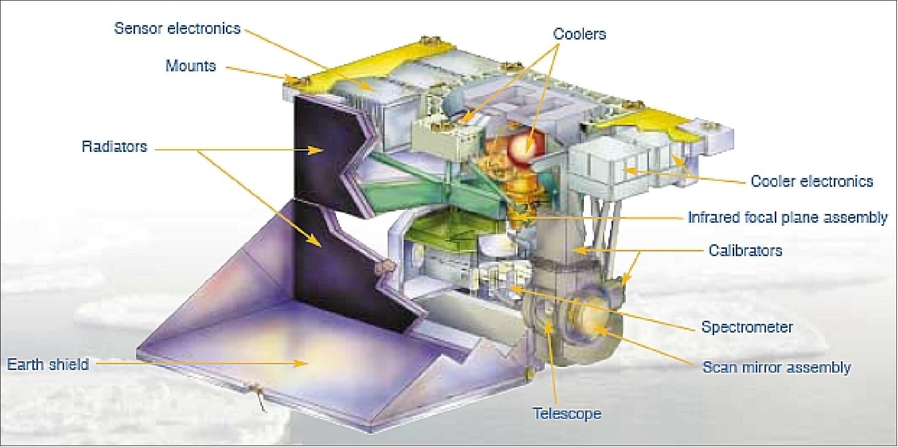
The AIRS spectrometer is a pupil imaging, multi-aperture echelle grating design that utilizes a coarse 13 lines/mm grating at high orders (3-11) to disperse infrared energy across a series of detector arrays. The typical entrance slit of a spectrometer is subdivided into a series of eleven apertures, each of which is imaged onto the focal plane. The grating serves to spectrally disperse each image, which in turn is overlaid onto a HgCdTe detector array with each detector in the array viewing a unique wavelength by virtue of the grating dispersion. Rejection of overlapping grating orders and background photon suppression is provided by a series of IR bandpass filters located within the spectrometer and directly on the focal plane. Use of the grating in combination with the filter set provides a two-dimensional color map on the focal plane with a high degree of design flexibility in terms of color arrangement and spacing. Cooling of the spectrometer to 155 K is provided by a two stage passive radiator assembly with 10 Watt cooling capacity at 155 K.
Dispersed energy exiting the spectrometer is imaged onto a state-of-the-art hybrid PV/PC: HgCdTe focal plane assembly (FPA) consisting of a series of multi-linear arrays each associated with a specific entrance aperture. The assembly consists of 17 arrays arranged in 12 modules with each module individually optimized for wavelength and photon flux. The module set includes 10 photovoltaic (PV) modules covering the 3.7 - 13.7 µm region and 2 photoconductive (PC) modules for the 13.7 - 15.4 µm region. The more advanced PV modules include on-focal plane signal processing via a custom CMOS Readout IC (ROIC) specifically designed for AIRS temperature, photon flux and radiation conditions. The ROIC provides the first stage of signal integration at a 1.4 ms subsample rate, which are summed off focal plane in groups of 16 to meet full footprint dwell time requirements. The IR FPA provides simultaneous measurement of 2378 spectral samples across the 3.7 - 15.4 µm region with two samples per resolution element. Additionally, each PV sample is further divided by two in the cross-dispersed direction to provide increased yield and a measure of spectral redundancy. As a consequence, the IR FPA contains a total of 4482 active detectors. The complex FPA is packaged in a vacuum dewar maintained at the 155 K spectrometer operating temperature, with the IR FPA cooled to 58 K via a redundant, 1.5 W capacity Split Stirling pulse tube cryocooler.

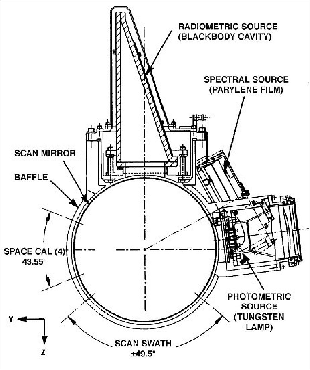
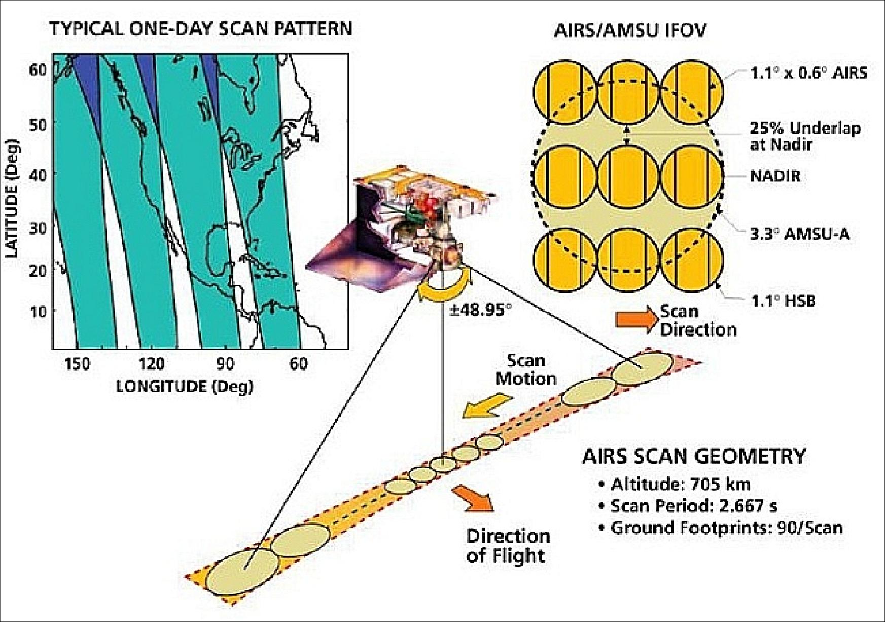
The infrared region of 3.74-15.4 µm has a spectral resolution of 1200 (lambda/ delta lambda). The high spectral resolution permits the separation of unwanted spectral emissions and, in particular, provides spectrally clean “super windows,” ideal for surface observations. - This is supplemented by a VNIR photometer of four bands in the range between 0.4 and 1.0 µm. The VNIR channels are used to discriminate between low-level clouds and different terrain and surface covers, including snow and ice. The AIRS infrared bands have an IFOV of 1.1º and FOV = ± 49.5º scanning capability perpendicular to the spacecraft ground track (swath width = 1650 km, 13.5 km horizontal resolution in nadir, 1 km vertical). It takes 22.41 ms for each footprint of 1.1º in diameter (or 13.5 km). Each IR scan produces 90 footprints across the flight track and takes 2.67 s (see Figure 56). The VNIR channels have a footprint of 0.185º or about 2.3 km on the ground, nine VNIR footprints are within a 40 km swath. The VNIR photometer is boresighted to the spectrometer to allow simultaneous VNIR observations.
The VNIR photometer uses optical filters to define the four spectral bands. It operates at ambient temperatures (293-300 K). Inflight calibration is performed during each scan period. In addition, AIRS uses four independent cold-space views.
The major data products derived from AIRS are atmospheric temperature profiles, humidity profiles (from channels in the 6.3 µm water vapor band and the 11 µm windows, sensitive to the water vapor continuum), and land skin surface temperature.
AIRS is flown on the Aqua satellite with two operational microwave sounders: NOAA's AMSU and Brazil's HSB (Humidity Sounder Brazil). Together, the three sensors constitute constitute a possible advanced operational sounding system for future NOAA missions - offering increased accuracy of short-term weather predictions, improved tracking of severe weather events like hurricanes, and advances in climate research.
Instrument type | Multi-aperture, non-Littrow echelle array grating spectrometer configuration |
Spectral coverage | 3.74 - 15.4 µm for the array grating spectrometer (IR bands) |
Spectral resolution | 1200 (lambda/delta lambda) array grating spectrometer, 2378 bands |
Spatial resolution | 13.5 km horizontal at nadir for IR bands (IFOV = 1.1º), 1 km vertical resolution, 2.3 km x 2.3 km for VNIR bands (IFOV = 0.185º) |
IR detector cooling | Two-stage passive radiative cooler with retractable earth shield, |
Swath width | 1650 km (FOV= ± 49.5º) for IR bands; 40 km for VNIR bands |
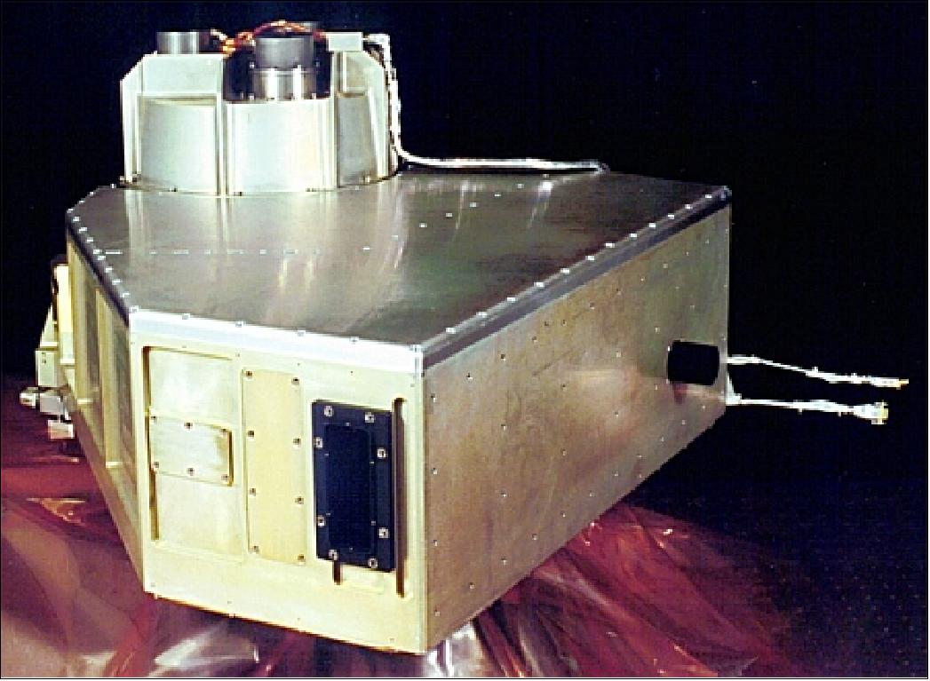
Instrument mass, power | 177 kg, 220 W |
Date rate, duty cycle | 1.27 Mbit/s, 100% |
Some AIRS results in 2010
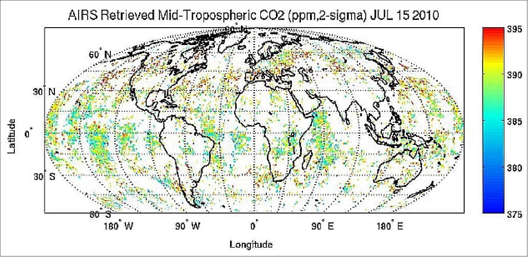
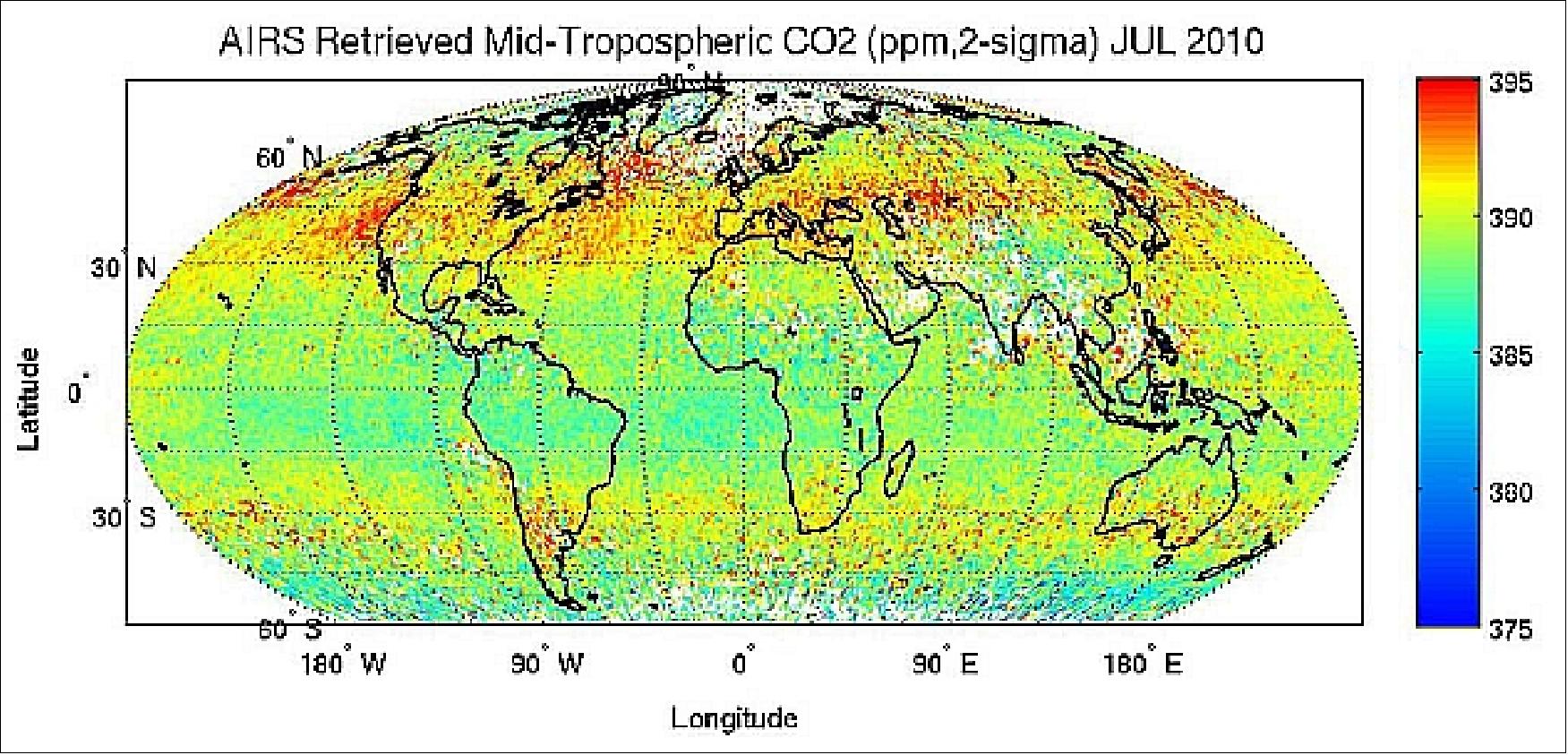
The excellent sensitivity and stability of the AIRS instrument has recently allowed the AIRS team to successfully retrieve Carbon Dioxide (CO2) concentrations in the mid-troposphere (8-10 km) with a horizontal resolution of 100 km and an accuracy of better than 2 ppm. 40)
Originally designed to retrieve temperature and water vapor profiles for weather forecast improvement, the AIRS (Atmospheric Infrared Sounder) has become a valuable tool for the measurement and mapping of mid-tropospheric carbon dioxide concentrations. Several researchers have demonstrated the ability to retrieve mid-tropospheric CO2 from AIRS by different methods. The retrieval method selected for processing and distribution is called the method of “Vanishing Partial Derivatives” and results in over 15,000 CO2 retrievals per 24-hour period with global coverage and an accuracy better than 2 ppm.
The AIRS CO2 accuracy has been validated against a variety of mid-tropospheric aircraft measurements as well as upward looking interferometers (FTIR) from the ground.
Mid-tropospheric CO2 concentrations are an indicator for atmospheric transport and several interesting findings have resulted from analysis of the data.
- First is the non-uniformity of CO2, primarily caused by weather.
- Second is the ability to identify stratospheric-tropospheric exchange during a sudden stratospheric warming event.
- Third is the presence of a seasonally varying belt of enhanced CO2 concentrations in the Southern Hemisphere.
Carbon dioxide turns out to be an excellent tracer gas since it does not react with other gases in the atmosphere. The project is finding that the AIRS mid-tropospheric CO2 is a good indicator of vertical motion in the atmosphere. It is a known fact that the majority of atmospheric CO2 is produced and absorbed near the surface and that there are no sources or sinks in the free troposphere. Thus elevated levels of mid-tropospheric CO2 are the result of airflow into the mid-troposphere from the near surface.
The most obvious finding from the AIRS retrievals is that the distribution of CO2 is not uniform as indicated in the models. Strong latitudinal and longitudinal gradients exist particularly over the large land masses in the Northern Hemisphere. This phenomenon is referred to as “CO2 weather”. The large variability in atmospheric circulation due to convection and global and mesoscale transport is responsible for most of the variability seen in the AIRS data. This implies that the AIRS CO2 data will be extremely useful for validating global scale transport in GCMs (Global Circulation Models).
AMSU/HSB
AMSU/HSB (Advanced Microwave Sounding Unit (NASA Instrument)/ (Humidity Sounder for Brazil), provided by INPE. Both instruments operate in conjunction.
AMSU was designed and developed by Aerojet of Azusa, CA (a GenCorp company). AMSU primarily provides temperature soundings, whereas HSB provides humidity soundings. AMSU is a 15-channel microwave radiometer. AMSU and HSB have a total of 19 channels, 15 are assigned to AMSU, each having a 3.3º beamwidth, and four are assigned to HSB, each having a beamwidth of 1.1º. AMSU comprises two separate units: AMSU-A1 (channels 3-15), and AMSU-A2 (channels 1 and 2). Channels 3 - 14 use the 50 to 60 GHz oxygen band to provide data for vertical temperature profiles up to 50 km. The “window” channels (1, 2, and 15) provide data to enhance the temperature sounding by correcting for surface emissivity, atmospheric liquid water, and total precipitable water. HSB channels 17 - 20 use the 183.3 GHz water vapor absorption line to provide data for the humidity profile. 41) 42)
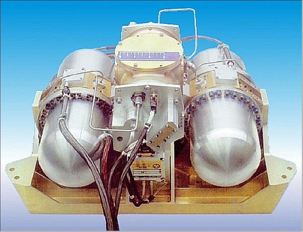
AMSU-A1 measures temperature profiles from the surface up to 50 km in 15 channels. Temperature resolution: 0.25 - 1.2 K. The AMSU-A1 instrument has two 15 cm diameter antennas (reflectors with momentum compensation), each with a 3.3º nominal IFOV at the half power points or FWHM (Full width Half maximum). Each antenna provides a cross-track scan of ±49.5º from nadir with a total of 30 Earth views (scan positions) per scan line. The total scan period is eight seconds. The footprint (resolution) at nadir is 40 km. The swath width is approximately 1690 km. Internal calibration is performed with internal warm loads and cold space.
AMSU-A2 has a single 28 cm diameter antenna (reflector without momentum compensation) with a 3.3º nominal IFOV. All other instrument/observation parameters are the same as those of AMSU-A1.
AMSU parameters: mass = 91 kg (49 kg for AMSU-A1, 42 kg for AMSU-A2); power = 101 W; data rate = 2.0 kbit/s; thermal control by heater, central thermal bus, radiator; thermal operating range= 0-20º C.
Sensor | Channel | Center Frequency (GHz) | Bandwidth (MHz) | Sensitivity NEΔT (K) |
AMSU-A2 | 1 | 23.8 | 280 | 0.3 |
AMSU-A1 | 3 | 50.300 | 180 | 0.4 |
HSB | 17 | 150.0 | 2000 | 1.0 |
Parameter | AMSU-A1 | AMSU-A2 |
Instrument size | 72 cm x 34 cm x 59 cm | 73 cm x 61 cm x 68 cm |
Mass, power | 49 kg, 72 W | 42 kg |
Data rate | 1.3 kbit/s | 0.4 kbit/s |
Antenna size | 15 cm (2 units) | 31 cm (1 unit) |
IFOV (Instantaneous Field of View) | 3.3º | 3.3º |
Swath width | 100º, 1650 km | 100º, 1650 km |
Pointing accuracy | 0.2º | 0.2º |
No of channels | 13 | 2 |
HSB (Humidity Sounder for Brazil)
HSB is an INPE-provided instrument of AMSU-B heritage (built by MMS (Matra Marconi Space) of Bristol, UK (now EADS Astrium Ltd) with participation of Equatorial Sistemas of Brazil), and sponsored by AEB (Brazilian Space Agency). HSB is a microwave radiometer with the objective to measure atmospheric radiation, to obtain atmospheric water vapor profile measurements and to detect precipitation under clouds with 13.5 km horizontal nadir resolution (humidity profiles for weather foresting). 43) 44) 45)
HSB is a four-channel self-calibrating instrument (passive sounder) providing a humidity profiling capability in the frequency range of 150 - 190 GHz, spanning the height from surface to about 42 km. The measured signals are also sensitive to a) liquid water in clouds (cloud liquid water content) and b) graupel and large water droplets in precipitating clouds (qualitative estimate of precipitation rate). HSB scans in the cross-track direction at a rate of 2.67 seconds in continuous mode. The instrument features a momentum-compensated scan mirror system. HSB is operated in combination with AMSU-A, they have a total of 19 channels: 15 are assigned to AMSU-A, each having a 3.3º beamwidth, and four assigned to HSB, each having a 1.1º beamwidth. The HSB receiver channels are configured to operate in DSB (Double Sideband).
The HSB collected valuable data for the first nine months of the mission but ceased operating in February 2003 (scanner anomaly).
Nr. of channels | 4 (total), Ch 17 at 150 GHz, Ch 18: 183.31 ±1 GHz, Ch. 19: 183.31 ±3 GHz, and Ch 20: 183.31 ±7 GHz |
Swath width, scan period | 1650 km, 2.67 s |
FOV | ±49.5º cross track from nadir (+90º to -49.5º for calibration) |
IFOV (spatial resolution) | 1.1º (13.5 km at nadir) |
Instrument pointing | Control = 3600 arcseconds, knowledge = 360 arcseconds, |
Thermal control, operating range | Radiator, 13 - 35ºC |
Instrument power | 80 W average, 154 W peak |
Instrument mass, size, data rate | 51 kg, 70 cm x 65 cm x 46 cm, 4.2 kbit/s |
Temperature accuracy (data profile) | 1.0 - 1.2 K, coverage (twice daily) of land and ocean surfaces, resolution of 50 km (horiz.) and 1 km (vertical), up to 100 mb |
Humidity accuracy (data profile) | 20%, global coverage (twice daily), res. = 50 km, 1 km (vertical) |
Radiance accuracy (data profile) | 1-1.2 K, global coverage (twice daily), res. = 15 km (average) |
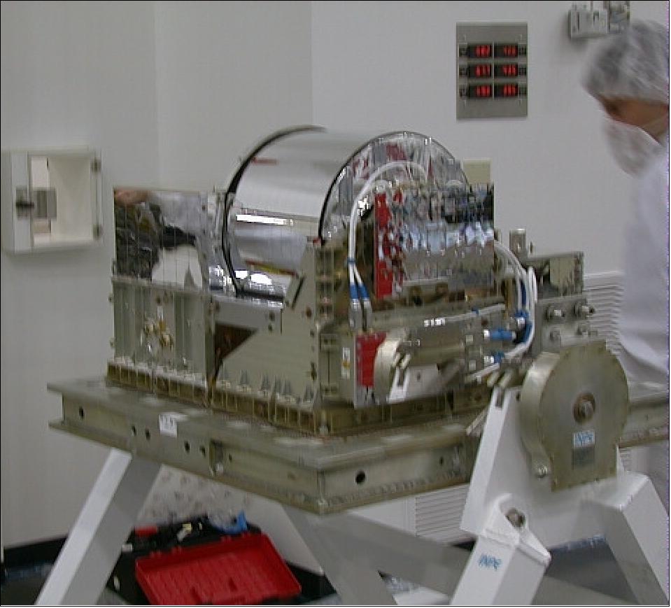
AMSR-E (Advanced Microwave Scanning Radiometer-EOS)
AMSR-E is a JAXA/NASA cooperative instrument, of AMSR heritage, built by Mitsubishi Electronics Corporation (PIs: A. Shibata, R. W. Spencer). The objective is the measurement of geophysical parameters such as: cloud properties, radiative energy flux, precipitation, land surface wetness (moisture), sea ice, snow cover, sea surface temperature (SST), and sea surface wind fields. AMSR-E is a modified design of AMSR on ADEOS-II (Japan).
The AMSR-E instrument is a conically scanning total power passive microwave radiometer sensing microwave radiation (brightness temperatures) at 12 channels and 6 frequencies ranging from 6.9 to 89.0 GHz (6.925, 10.65, 18.7, 23.8, 36.5, and 89.0 GHz). Horizontally and vertically polarized radiation are measured separately at each frequency. 46) 47) 48)
AMSR-E consists of an offset parabolic reflector 1.6 m in diameter, fed by an array of six feedhorns. The reflector and feedhorn arrays are mounted on a drum which contains the radiometers, digital data subsystem, mechanical scanning subsystem, and power subsystem. The reflector/feed/drum assembly is rotated about the axis of the drum by a coaxially mounted bearing and power transfer assembly. All data, commands, timing and telemetry signals, and power pass through the assembly on slip ring connectors to the rotating assembly. The AMSR-E instrument has a mass of 314 kg, power = 350 W, a duty cycle of 100%, and an average data rate of 87.4 kbit/s.
Center frequency (GHz) | 6.925 | 10.65 | 18.7 | 23.8 | 36.5 | 89.0 |
Bandwidth (MHz) | 350 | 100 | 200 | 400 | 1000 | 3000 |
Sensitivity (K) | 0.3 | 0.6 | 0.6 | 0.6 | 0.6 | 1.1 |
IFOV (km x km) footprint | 75 x 43 | 51 x 29 | 27 x 16 | 31 x 18 | 14 x 8 | 6 x 4 |
Sampling rate (km x km) | 10 x 10 | 10 x 10 | 10 x 10 | 10 x 10 | 10 x 10 | 5 x 5 |
Integration time (ms) | 2.6 | 2.6 | 2.6 | 2.6 | 2.6 | 1.3 |
Main beam efficiency (%) | 95.3 | 95.0 | 96.3 | 96.4 | 95.3 | 96.0 |
Beamwidth (º) | 2.2 | 1.4 | 0.8 | 0.9 | 0.4 | 0.18 |
Polarization | Horizontal and Vertical | |||||
Incidence angle | 55º | 54.5º | ||||
Cross polarization | < - 20 dB | |||||
Swath width | > 1450 km | |||||
Dynamic range | 2.7 - 340 K | |||||
Data quantization | 12 bit | 10 bit | ||||
Data rate | 87.4 kbit/s | |||||
Antenna size, control unit | 1.95 m x 1.7 m x 2.4 m, 0.8 m x 1.0 m x 0.6 m | |||||
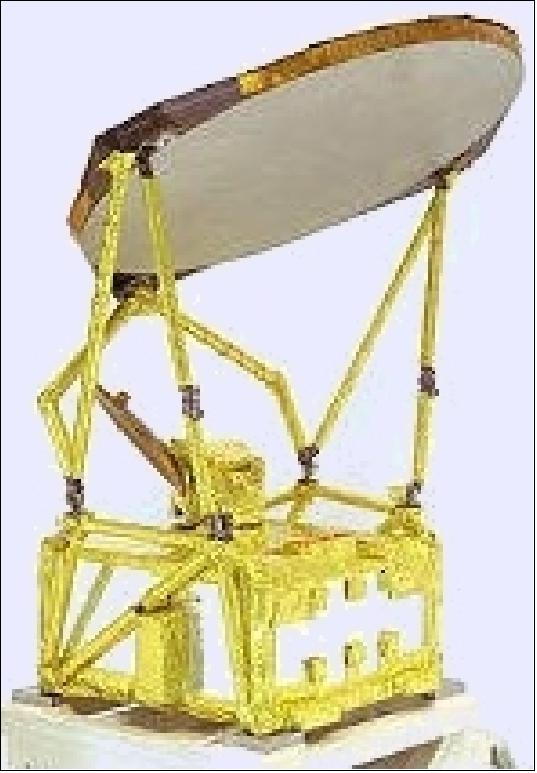
The AMSR-E instrument rotates continuously about an axis parallel to the local spacecraft vertical at 40 rpm. At an altitude of 705 km, it measures the upwelling scene brightness temperatures over an angular sector of ± 61º about the subsatellite track, resulting in a swath width of 1445 km. During a period of 1.5 seconds the S/C subsatellite point travels 10 km. Even though the IFOV for each channel is different, active scene measurements are recorded at equal intervals of 10 km (5 km for the 89 GHz channels) along the scan. The half cone angle at which the reflector is fixed is 47.4º which results in an Earth incidence angle of 55.0º.
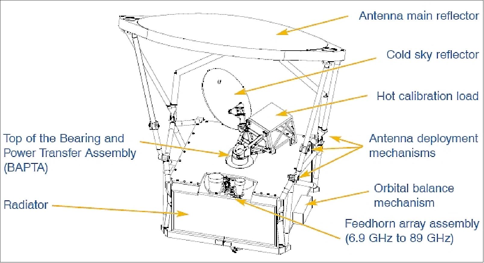
Instrument calibration. The radiometer calibration accuracy budget, exclusive of antenna pattern correction effects, is composed of three major contributors: warm load reference error, cold load reference error, radiometer electronics nonlinearities and errors.
Some data products from AMSR-E are:
• Level 2A brightness temperatures
• Level 2 rainfall
• Level 3 rainfall
• Columnar cloud water over the oceans
• Columnar water vapor over the oceans
• Sea surface temperature (SST)
• Sea surface wind speed
• Sea ice concentration
• Sea ice temperature
• Snow depth on sea ice
• Snow-water equivalent on land
• Surface soil moisture
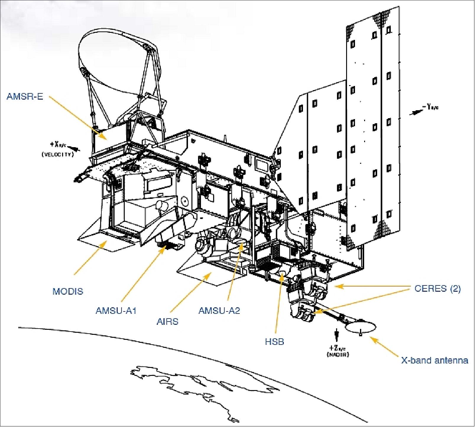
References
1) C. L. Parkinson, “Aqua: An Earth-Observing Satellite Mission to Examine Water and other Climate Variables,” IEEE Transactions on Geoscience and Remote Sensing, Vol. 41, No 2, Feb. 2003, pp. 173-183, Note: The entire issue is devoted to the EOS Aqua Mission.
3) http://www.nasa.gov/pdf/151986main_Aqua_brochure.pdf
4) Eric J. Fetzer, “Observing Clouds and Water Vapor with NASA's A-Train,” Joint GCSS-GPCI/BLCI-RICO Workshop, NASA/GISS New York, USA, Sept. 18, 2006, URL: http://www.knmi.nl/samenw/rico/presentations/Fetzer_GCSS.pdf
5) ”Smoke Over Siberia,” NASA Earth Observatory, Image of the Day for 19 July 2022, URL: https://earthobservatory.nasa.gov/images/150097/smoke-over-siberia
6) ”Floods Swamp Bangladesh,” NASA Earth Observatory, Image of the Day for 24 June 2022, URL: https://earthobservatory.nasa.gov/images/150014/floods-swamp-bangladesh
7) ”Alaska Ablaze,” NASA Earth Observatory, Image of the Day for 15 June 2022, URL: https://earthobservatory.nasa.gov/images/149973/alaska-ablaze
8) ”Phytoplankton Productivity Down in Gulf of Maine,” NASA Earth Observatory, Image of the Day for 8 June 2022, URL: https://earthobservatory.nasa.gov/images/149915/phytoplankton-productivity-down-in-gulf-of-maine
9) ”Bristol Abloom,” NASA Earth Observatory, Image of the Day for 4 June 2022, URL: https://earthobservatory.nasa.gov/images/149912/bristol-abloom
10) AbigailMcQuatters-Gollop, Angus Atkinson, Anaïs Aubert, Jacob Bedford, Mike Best, Eileen Bresnan, Kathryn Cook, Michelle Devlin, Richard Gowen, David G. Johns, Margarita Machairopoulou, April McKinney, Adam Mellor, Clare Ostle, Cordula Scherer, Paul Tett, ”Plankton lifeforms as a biodiversity indicator for regional-scale assessment of pelagic habitats for policy,” ScienceDirect, Volume 10, June 2019, pp: 913-925, https://doi.org/10.1016/j.ecolind.2019.02.010
11) ”Persistent Dust Storms Batter Iraq, NASA Earth Observatory, Image of the Day for 18 May 2022, URL: https://earthobservatory.nasa.gov/images/149838/persistent-dust-storms-batter-iraq
12) ”New Mexico Wildfire Spawns Fire Cloud,” NASA Earth Observatory, Image of the Day for 14 May 2022, URL: https://earthobservatory.nasa.gov/images/149830/new-mexico-wildfire-spawns-fire-cloud
13) ”Taking Stock of Rocky Mountain Snowpack,” NASA Earth Observatory, Image of the Day for 6 May 2022, URL: https://earthobservatory.nasa.gov/images/149779/taking-stock-of-rocky-mountain-snowpack
14) A. Park Williams, Benjamin I. Cook & Jason E. Smerdon, ”Rapid intensification of the emerging southwestern North American megadrought in 2020–2021,” Nature Climate Change, Volume 12, pp: 232-234, Published: 14 February 2022, https://doi.org/10.1038/s41558-022-01290-z
15) ”From Weather Forecasting to Climate Change, NASA’s AIRS Builds a Legacy,” NASA/JPL, 5 May 2022, URL: https://www.jpl.nasa.gov/news/from-weather-forecasting-to-climate-change-nasas-airs-builds-a-legacy?utm_source=iContact&utm_medium=email&utm_campaign=nasajpl&utm_content=daily20220505-3
16) ”Wildfires Continue to Burn Across New Mexico,” NASA Earth Observatory, Image of the Day for 4 May 2022, URL: https://earthobservatory.nasa.gov/images/149784/wildfires-continue-to-burn-across-new-mexico
17) ”Mediterranean Dust Storm,” NASA Earth Observatory, Image of the Day for 2 May 2022, URL: https://earthobservatory.nasa.gov/images/149772/mediterranean-dust-storm
18) ”Picturesque Clouds off Greenland,” NASA Earth Observatory, Image of the Day for 28 April 2022, URL: https://earthobservatory.nasa.gov/images/149759/picturesque-clouds-off-greenland
19) ”Wildfires Scorch Northern New Mexico,” NASA Earth Observatory, Image of the Day for 26 April 2022, URL: https://earthobservatory.nasa.gov/images/149748/wildfires-scorch-northern-new-mexico
20) Yizhou Zhuang, Rong Fu, Benjamin D. Santer, Robert E. Dickinson, and Alex Hall, ”Quantifying contributions of natural variability and anthropogenic forcings on increased fire weather risk over the western United States,” PNAS, Vol. 118 No 45, November 1, 2021, https://doi.org/10.1073/pnas.2111875118
21) ”A Grand New Dam on the Nile,” NASA Earth Observatory, Image of the Day for 19 April 2022, URL: https://earthobservatory.nasa.gov/images/149691/a-grand-new-dam-on-the-nile
22) Essam Heggy, Zane Sharkawy and Abotalib Z Abotalib, ”Egypt's water budget deficit and suggested mitigation policies for the Grand Ethiopian Renaissance Dam filling scenarios,” Environmental Research Letters, Volume 16, Number 7, Published: 1 July 2021, https://doi.org/10.1088/1748-9326/ac0ac9, URL: https://iopscience.iop.org/article/10.1088/1748-9326/ac0ac9/pdf
23) Prakrut Kansara, Wenzhao Li, Hesham El-Askary, Venkataraman Lakshmi, Thomas Piechota, Daniele Struppa and Mohamed Abdelaty Sayed,”An Assessment of the Filling Process of the Grand Ethiopian Renaissance Dam and Its Impact on the Downstream Countries,” Remote Sensing, Published: 15 February 2021, https://doi.org/10.3390/rs13040711, URL: https://mdpi-res.com/d_attachment/remotesensing/remotesensing-13-00711/article_deploy/remotesensing-13-00711-v2.pdf
24) ”Dry Winds and Grasses Fuel Texas Fires,” NASA Earth Observatory, Image of the Day for 22 March 2022, URL: https://earthobservatory.nasa.gov/images/149608/dry-winds-and-grasses-fuel-texas-fires
25) ”A Salt Bath in Bolivia,” NASA Earth Observatory, Image of the Day for 28 February 2022, URL: https://earthobservatory.nasa.gov/images/149502/a-salt-bath-in-bolivia
26) ”Cyclone Batsirai Floods Madagascar,” NASA Earth Observatory, Image of the Day for 13 February, 2022, URL: https://earthobservatory.nasa.gov/images/149454/cyclone-batsirai-floods-madagascar
27) ”Blizzard Blankets Northeast U.S. in Snow,” NASA Earth Observatory, Image of the Day for 1 February 2022, URL: https://earthobservatory.nasa.gov/images/149402/blizzard-blankets-northeast-us-in-snow
28) ”Suspended Sediments Streak a Shallow Gulf,” NASA Earth Observatory, Image of the Day for 29 January 2022, URL: https://earthobservatory.nasa.gov/images/149359/suspended-sediments-streak-a-shallow-gulf
29) ”Flash Floods Swamp Iran,” NASA Earth Observatory, Image of the Day for 15 January 2022, URL: https://earthobservatory.nasa.gov/images/149325/flash-floods-swamp-iran
30) ”Red Tide off Rio,” NASA Earth Observatory, Image of the Day for January 13, 2022, URL: https://earthobservatory.nasa.gov/images/149316/red-tide-off-rio
31) ”Colorado Faces Winter Urban Firestorm,” NASA Earth Observatory, Image of the Day for 5 January 2022, URL: https://earthobservatory.nasa.gov/images/149286/colorado-faces-winter-urban-firestorm
32) http://aqua.nasa.gov/about/instruments.php
33) H. H. Aumann, M. Chahine, C. Gautier, M. D. Goldberg, E. Kalnay, L. M. McMillin, H. Revercomb, P. W. Rosenkranz, W. L. Smith, D. H. Staelin, L. L. Strow, J. Susskind, “AIRS/AMSU/HSB on the Aqua Mission: Design, Science Objectives, Data Products, and Processing Systems,” IEEE Transactions on Geoscience and Remote Sensing, Vol. 41, No 2, pp. 253-264, February 2003, URL http://www.geog.ucsb.edu/~gautier/CV/pubs/Auman_et_al_2003.pdf
34) Aqua brochure of NASA/GSFC, March 2002, courtesy of Claire L. Parkinson, URL: http://aqua.nasa.gov/doc/pubs/Aqua_brochure.pdf
35) http://www-airs.jpl.nasa.gov/
36) M. H. Weiler, K. R. Overoye, J. A. Stobie, P. B. O'Sullivan, S. L. Gaiser, S. E. Broberg, D. A. Elliott, “Performance of the Atmospheric Infrared Sounder (AIRS) in the Radiation Environment of Low-Earth Orbit,” Proceedings of the SPIE Conference Optics and Photonics, San Diego CA, USA, July 31-Aug. 4, 2005, Vol. 5882
37) C. D. Barnet, M. D. Goldberg, L. McMillin, M. T. Chahine, “Remote sounding of trace gases with the EOS/AIRS instrument,” `Atmospheric and Environmental Remote Sensing Data Processing and Utilization: an End-to-End System Perspective,' Edited by Huang, Hung-Lung A.; Bloom, Hal J. Proceedings of the SPIE, Vol. 5548, 2004, pp. 300-312
38) http://aqua.nasa.gov/about/instrument_airs.php
39) Stuart MacCallum, “The Atmospheric InfraRed Sounder,” 2005, URL: http://xweb.geos.ed.ac.uk/~stuart/Presentations/stuart_firbush2005.pdf
40) Thomas S. Pagano, Moustafa T. Chahine, Edward T. Olsen, “Seven years of observations of Mid-Tropospheric CO2 from the Atmospheric Infrared Sounder,” Proceedings of the 61st IAC (International Astronautical Congress), Prague, Czech Republic, Sept. 27-Oct. 1, 2010, IAC-10.B1.6.3
41) Eric Fetzer, Larry M. McMillin, David Tobin, Hartmut H. Aumann, Michael R. Gunson, W. Wallace McMillan, Denise E. Hagan, Mark D. Hofstadter, James Yoe, David N. Whiteman, John E. Barnes, Ralf Bennartz, Holger Vömel, VonWalden, Michael Newchurch, Peter J. Minnett, Robert Atlas, Francis Schmidlin, Edward T. Olsen, Mitchell D. Goldberg, Sisong Zhou, HanJung Ding, William L. Smith, and Hank Revercomb “AIRS/AMSU/HSB validation,” IEEE Transactions on Geoscience and Remote Sensing, Vol. 41, Issue 2, Feb. 2003, pp. 418-431
42) Eric J. Fetzer, Edward T. Olsen, Luke Chen, Denise Hagan, “Validation of AIRS / AMSU / HSB retrieved products,” URL: http://trs-new.jpl.nasa.gov/dspace/bitstream/2014/38290/1/03-1851.pdf
43) Information provided by Janio Kono of INPE, Sao José dos Campos, Brazil
44) B. H. Lambrigtsen, R. V. Calheiros, “The Humidity Sounder for Brazil - an international partnership,” IEEE Transaction on Geoscience and Remote Sensing, Vol. 41, Issue 2, Feb. 2003, pp. 352-361
45) Ezio Castejon Garcia, Marcio Bueno dos Santos, “The Environmental Simulation of the Humidity Sounder for Brazil,” 54th Astronautical Congress of the IAF, Sept. 29 - Oct. 3, 2003, Bremen, Germany
46) http://www.ghcc.msfc.nasa.gov/AMSR/instrument_descrip.html
47) AMSR-E Data Users Handbook, 4th Edition, JAXA, March 2006, NCX-030021
48) http://nsidc.org/data/docs/daac/amsre_instrument.gd.html
The information compiled and edited in this article was provided by Herbert J. Kramer from his documentation of: ”Observation of the Earth and Its Environment: Survey of Missions and Sensors” (Springer Verlag) as well as many other sources after the publication of the 4th edition in 2002. - Comments and corrections to this article are always welcome for further updates (eoportal@symbios.space).
Spacecraft Launch Mission Status Sensor Complement References Back to top