ERS-2 (European Remote-Sensing Satellite-2)
EO
ESA
Atmosphere
Ocean
Launched in April 1995, the ERS-2 was an enhancement of the previous ERS-1 mission. ERS-2 provided microwave spectrum environmental monitoring across a range of disciplines (oceans, polar ice, forestry).
Quick facts
Overview
| Mission type | EO |
| Agency | ESA |
| Mission status | Mission complete |
| Launch date | 21 Apr 1995 |
| End of life date | 04 Jul 2011 |
| Measurement domain | Atmosphere, Ocean, Land, Gravity and Magnetic Fields, Snow & Ice |
| Measurement category | Cloud type, amount and cloud top temperature, Aerosols, Multi-purpose imagery (ocean), Radiation budget, Multi-purpose imagery (land), Surface temperature (land), Vegetation, Albedo and reflectance, Gravity, Magnetic and Geodynamic measurements, Surface temperature (ocean), Atmospheric Humidity Fields, Ozone, Trace gases (excluding ozone), Landscape topography, Ocean topography/currents, Sea ice cover, edge and thickness, Soil moisture, Snow cover, edge and depth, Ocean surface winds, Ocean wave height and spectrum, Ice sheet topography |
| Measurement detailed | Ocean imagery and water leaving spectral radiance, Aerosol absorption optical depth (column/profile), Cloud cover, Aerosol optical depth (column/profile), Cloud type, Land surface imagery, Vegetation type, Earth surface albedo, Downwelling (Incoming) solar radiation at TOA, Short-wave Earth surface bi-directional reflectance, Atmospheric specific humidity (column/profile), O3 Mole Fraction, Land surface temperature, Sea surface temperature, Land surface topography, Wind vector over sea surface (horizontal), NO2 Mole Fraction, Sea-ice cover, Snow cover, Soil moisture at the surface, Wind speed over sea surface (horizontal), BrO (column/profile), Sea-ice thickness, Significant wave height, Bathymetry, Geoid, Dominant wave direction, Sea level, OClO (column/profile), Sea-ice type, Glacier motion, Ocean dynamic topography, Dominant wave period, SO2 Mole Fraction, Sea-ice sheet topography |
| Instruments | MWR, ATSR/M, AMI/SAR/Image, AMI/Scatterometer, ERS Comms, AMI/SAR/Wave, RA, GOME, ATSR-2 |
| Instrument type | Imaging multi-spectral radiometers (vis/IR), Scatterometers, Atmospheric chemistry, Communications, Imaging multi-spectral radiometers (passive microwave), Radar altimeters, Imaging microwave radars |
| CEOS EO Handbook | See ERS-2 (European Remote-Sensing Satellite-2) summary |
Related Resources
Summary
Mission Capabilities
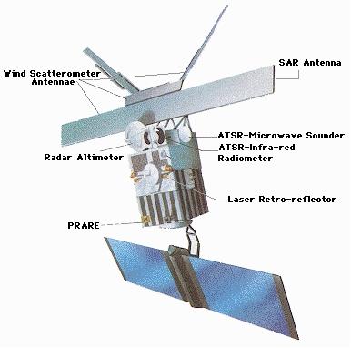
Sensors found on ERS-2 included the Active Microwave Instrument (AMI), Radar Altimeter-1 (RA-1), Along-Track Scanning Radiometer and Microwave Sounder-2 (ATSR-2), Laser Retro-Reflector (LRR), Precise Range and Range-Rate Equipment (PRARE) and Global Ozone Monitoring Experiment (GOME).
AMI, RA-1, LRR and PRARE were carried over from the preceding ERS-1 mission, with ATSR-2 updated for the ERS-2 mission.
GOME was added to ERS-2 to complete its sensor complement. AMI was a dual-radar which utilised three modes to detect different phenomena on Earth. This included Imaging mode, where C-band measurements were used to conduct imagery of the Earth. Other modes included wave mode, where the reflectivity of the sea surface caused by surface waves could be processed to identify the length and direction of wave systems, and wind scatterometer mode (SCAT) which used three different antennas to measure sea surface wind speed and direction. RA-1 operated in Ku-band with two modes, ocean and ice mode, which provided various ice parameters, wave height, ocean surface elevation for tide and current studies, and ocean surface wind speeds.
LRR was mainly used to ensure the accuracy of satellite tracking from the ground, while PRARE was used for orbit determination and ionospheric corrections to ensure accurate data collection. ATSR-2 was updated with increased spectral band imaging to provide data for vegetation studies in addition to existing data on sea surface temperature for climate change scientists.
Lastly, GOME was added to observe upwelling solar radiation reflected or scattered in Earth’s atmosphere and from its surface.
Performance Specifications
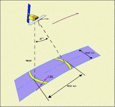
The spatial resolution was dependent on the operational mode of AMI. In imaging mode, the spatial resolution was 30 m with a swath width of 100 km and an incidence angle of 23°. In wave mode, the spatial resolution was also 30 m however with a greater swath width of 5 km x 5 km, while the scatterometer mode yielded a spatial resolution of 50 km and a swath width of 500 km, with a variable incidence angle.
Imaging was completed using a singular C-band frequency wave. ATSR-2 was able to measure in 7 bands between Visible (VIS) and Thermal Infrared (TIR) ranges.
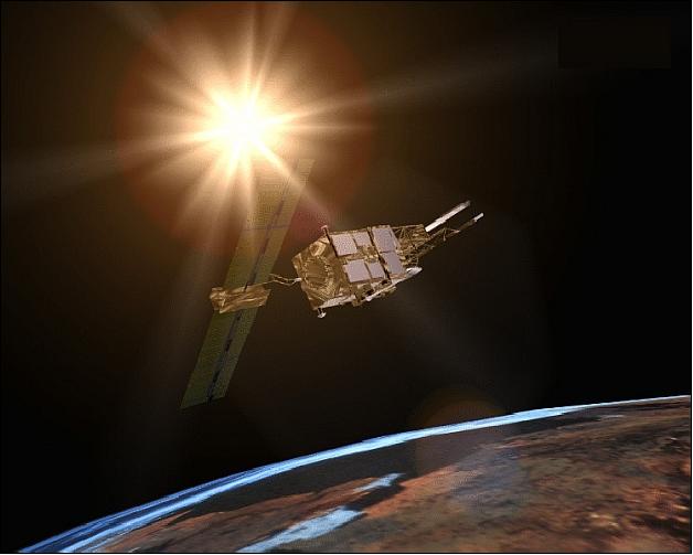
ERS-2 operated in a sun-synchronous polar orbit at a mean altitude of 780 km and an inclination angle of 98.5°. The orbital period was 100 minutes with a revisit time of 35 days.
Space and Hardware Components
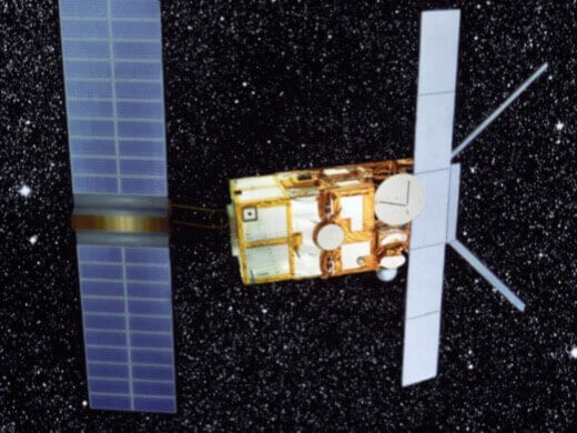
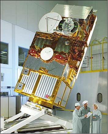
The bus used for ERS-2 was the SPOT MK1 bus, based on the SPOT Multimission Platform used for ERS-1. The bus included a service module, propulsion module, payload module and a dual-wing solar array subassembly.
Furthermore, ground systems were in place to support the satellite’s control and operation, specifically to archive and process instrument data and to satisfy user requirements. These ground stations were located in Italy, Spain and Canada, with the mission control centre in Darmstadt, Germany and system monitoring in Frascati, Italy.
The mission was terminated in 2011 to avoid the satellite ending up as space debris due to the risk of onboard power loss at any time, and to mitigate the risk of colliding with other satellites.
ERS-2 (European Remote-Sensing Satellite-2)
ERS-2 was the follow-up ESA mission of ERS-1. It was in 1989 when ESA decided to continue the ERS program beyond the lifetime of ERS-1.
The ERS-2 satellite was essentially a copy of ERS-1, except that it included a number of enhancements; it was also carrying a new payload instrument to measure the chemical composition of the atmosphere, named GOME (Global Ozone Monitoring Experiment).
ERS-2 had a total mass of 2,516 kg at launch (about 200 kg more than ERS-1). The mission design life requirement was extended to 3 years. ERS-2 had also the same mission objectives as ERS-1, plus an atmospheric chemistry mission objective (with GOME). 1) 2)
The description of the ERS-2 spacecraft and of the common sensor complement can be found under the ERS-1 description.
Launch
The launch of the ERS-2 spacecraft took place on April 21, 1995, from Kourou on an Ariane-4 vehicle.
Orbit:
Sun-synchronous polar orbit (retrograde orbit). Altitude = 780 km (mean); inclination = 98.5º, local crossing time of the equator = 10:30 AM, orbital period is about 100 minutes. Repeat cycle = 3 days or 35 days.
Mission Status
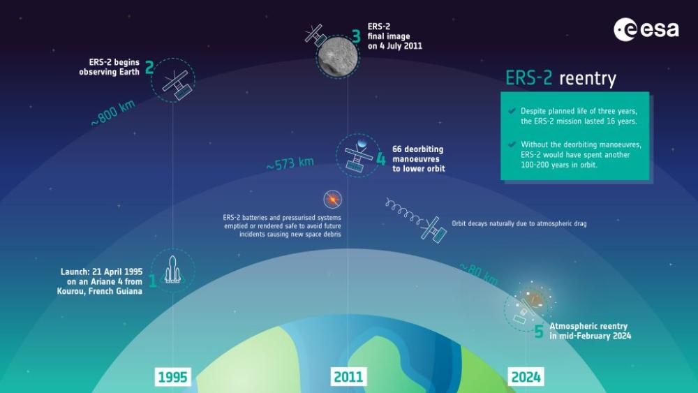
• February 21, 2024: At approximately 18:17 CET (17:17 UTC) ESA’s ERS-2 satellite completed its atmospheric reentry over the North Pacific Ocean, between Alaska and Hawaii. No damage to property has been reported.
Having far exceeded its planned lifetime of three years, ESA took the decision to deorbit ERS-2 in 2011 in light of growing concern over the long-term hazard that orbital debris poses to current and future space activities.The satellite’s altitude had been declining steadily ever since. On 21 February 2024, it reached the critical altitude of around 80 km at which the atmospheric drag was so strong that it began to break into pieces.
An international campaign involving the Inter-Agency Space Debris Coordination Committee and ESA’s Space Debris Office monitored the reentry. 46)
• February 5, 2024: ESA announced that ERS-2 reentry is predicted between February 16 and 22, 2024. 45)
• The ERS-2 mission ended on Sept. 5, 2011, after the satellite's average altitude had already been lowered from 785 km to about 573 km. At this height, the risk of collision with other satellites or space debris is greatly reduced.
- The final critical step was to 'passivate' ERS-2, ensuring that all batteries and pressurised systems were emptied or rendered safe in order to avoid any future explosion that could create new space debris. This primarily consisted of burning off the fuel, disconnecting the batteries and switching off the transmitters.
With the effects of natural atmospheric drag, ERS-2 is predicted to enter and largely burn up in the atmosphere in about 15 years. This is well within the 25-year limit that is imposed to minimise the risk of collision before reentry. 3)
• ESA retired the ERS-2 spacecraft in early July 2011 to avoid ending up with the mission as a piece of space debris. ERS-2 has been delivering data right to the end.
After orbiting Earth almost 85,000 times, the risk that the satellite could lose power at any time was clearly high. The deorbiting procedures were started on July 6, 2011, at ESOC with the goal to lower the satellite's orbit from its current altitude of 800 km to about 550 km, where the risk of collision is minimal. Eventually, ERS-2 will enter Earth's atmosphere and burn up.
ERS-2 spent 16 years in orbit, gathering a wealth of data that has revolutionized our understanding of Earth. This pioneering mission has not only advanced science but also forged the technologies we now rely on for monitoring our planet. 4)
• The ERS-2 spacecraft is “operating nominally” in early 2011 (the approved mission extension goes up to the end of 2011).
However, ERS-2 will cease its operations in mid-2011, after 16 years of successful activity. Preparations for the subsequent decommissioning and deorbiting have started. Before the end of its mission, ERS-2 is being exploited to the maximum of its capabilities, within the constraints of its ageing equipment. Until the Envisat orbital change of October 2010, ERS-2 was used for specific SAR Interferometry (InSAR) campaigns in tandem with Envisat.
- A new ERS-2 mission phase, with a three-day repeat cycle, is being prepared for the few months before the end of the mission. This phase will repeat the ERS-1 Ice Phases of 1992 and 1994, almost 20 years later, taking advantage of the availability of a GPS network supporting atmospheric corrections for InSAR applications. 5)
• Adding to their unique information from previous tandem missions, ESA’s ERS-2 and Envisat satellites have been paired up again – for the last time. Data from this final duet are generating 3D models of glaciers and low-lying coastal areas. 6)
The fourth tandem interferometric campaign, from July to October 2010, focused on low-lying coastal areas, such as New Orleans in the USA and the Po River Mouth in Italy. This information will be used for various applications in many different fields, in particular for creating accurate DEMs of coastal areas that could be used to help manage floods.
• On April 21, 2010, the ERS-2 celebrated its 15th anniversary on orbit. 7)
• The ERS-2 spacecraft is “operating nominally” in early 2010, more than 14.5 years after launch (nominal mission life of 3 years). A mission extension was approved to the end of 2011. 8) 9) 10) 11)
- The S/C performs gyroless operations since mid-2001
- The gyroless data are being Doppler screened removing the attitude uncertainty
- The SAR instrument works satisfactorily
- In June 2003, ERS-2 lost its onboard data storage capability, effectively ending its global coverage capability. However, a network of SAR data acquisition stations provides good coverage (real-time data reception).
In 2009, the ERS-1 and ERS-2 missions have a cumulative 18 years of ERS-1/2 data in the archive, representing the most complete and consistent SAR archive.
• Envisat / ERS-2 SAR tandem interferometry missions.
The objective was to:
a) measure the velocity of fast-moving polar glaciers (> 200 m/year). ERS/Envisat SAR data should be suited to map velocities of 1 cm between the two 30-minute passes,
b) to generate accurate low-relief Digital Elevation Models.
This is of particular interest for many low-elevation delta regions, in particular for polar areas (North Canada, North Russia) where there is no available SRTM DEM information. 12) 13)
- The second tandem mission started on Nov. 23, 2008, and ended in late April 2009 (both spacecraft acquired data over the same area just 28 minutes apart). The second campaign was due to end in late January 2009 but could be extended through to late April 2009 due to the excellent performance of the satellites and the strong teamwork between the mission data teams at ESRIN, and ESOC.
- After the completion of the tandem mission, ERS-2 drifted naturally (without manoeuvring) to its reference orbit.
The second tandem mission also had perfect timing due to the occurrence of low solar activity, which is very favourable for ERS-2 attitude stability, and the fact that ERS-2 could be left to quickly drift back to its nominal orbit without using additional resources. 14)
- The first SAR tandem mission took place from September 2007 to February 14, 2008. This required a temporal modification of the ERS-2 orbit (2 km offset versus nominal ground track) to have optimal interferometric baselines between ERS-2 and Envisat (30 min. separation).
• Status of the PRARE mission:
On Dec. 31, 2007, the fully functional onboard PRARE instrument was retired. The reason: The design of the PRARE ground segment was conceived for an operational period of 4 years; only a lot of 29 ground stations were provided on a global scale. After the German national funding ran out at the end of 2002, it became increasingly difficult to operate the PRARE system when ground stations experienced a hardware failure. Eventually, this resulted in 2 fully functional ground stations at the end of 2006. As a consequence, the PRARE instrument was switched off at the end of 2007. 15)
• Instrument and spacecraft performance reviews took place in December 2006 with the main outcome that ERS-2 can be operated for several years - assuming that measures compensating for ageing are being applied during 2007. The AOCS continues to be operated in Zero-Gyro mode for “fine mode” support and in the mono-gyro mode for the “coarse mode” support. The AMI SAR instrument is now being operated with an average duty cycle of 3.5 minutes per orbit.
• In late 2007, ESA approved a 3-year extension of the ERS-2 mission operations to the end of 2011. In 12 years of operations, only 50% of the onboard fuel had been used (hence, a further extension might be granted). Since Sept. 2007, the ERS-2 orbit has been shifted for a four-month trial of 30-minute ERS- Envisat interferograms (although this only works for high northern latitudes). One successful application has been measuring the fastest glacier in the world (14 km/year in Greenland) which could not be measured previously.
• The ERS-2 spacecraft reached 10 years in orbit on April 21, 2005, a remarkable engineering achievement. All platform subsystems and payload instruments are working “nominally” and are providing good data.
Close collaboration between ESA and EADS Astrium resulted in the successful implementation of a gyroless or ZGM (Zero-Gyro Mode) of operation. The ZGM software was loaded on June 6, 2001, and activated onboard. The first period of recommissioning lasted until the end of July 2001. In Nov. 2001, the tuning was improved to cover all data products. The ZGM represents a re-design of AOCS, making extended use of the platform's sensors and actuators to compensate for the lack of gyroscopes. The goal is to extend the ERS-2 mission until MetOp-1 becomes operational in 2006.
However, one consequence of renewed ERS-2 operations is that ATSR-2 high-rate operations are suspended since the Wind/Wave mode is used for S/C attitude control (only within narrow limits can the ATSR-2 HR mode be operated).
• In June 2003, ERS-2 lost its onboard data storage capability, effectively ending its global coverage capability (tape recorder A stopped functioning June 22, 2003, while tape recorder B failed Dec. 20, 2002). - This implied that only real-time observations could be supported starting by the end of June 2003.
From now on, the spacecraft returns data when in line of sight of an appropriately equipped ground station. And because the majority of such stations are found around Europe and Canada, ensuring good observation of the North Atlantic, ERS-2 coverage of these regions has been able to continue.
• Some control mode changes were required after the failure of the onboard tape recorders. The new strategy, referred to as R-YCM (Regional Yaw Control Monitoring) is based on a limited set of data. Orbit and attitude control are sufficient to support ERS-2 data use.
However, there are some limitations to InSAR use. 16) 17)
• The ERS-2 satellite was piloted in the nominal yaw steering mode, using 3 gyroscopes out of 6 available, from launch until Feb. 2000. During this period, there were several problems with the gyroscopes. [in 1997, the S/C lost gyro #2 and in 1998 a pointing anomaly on gyro #3 made it unreliable]. The measures implemented in Feb. 2000 to protect the satellite against further gyroscope failures have allowed the continuation of the ERS-2 operations, despite two major anomalies that took place in Jan. 2001 (during this period, the S/C was piloted using one gyroscope).
Under normal conditions, these would have meant the end of the ERS-2 mission, but the measures implemented meant that the effects were limited to the interruption of service for about one month and temporary degradation of data quality. 18) 19) 20)
Sensor Complement
The descriptions of AMI, RA-1 and LRR can be found under the ERS-1 mission. Here, only ATSR-2, GOME and PRARE are being described.
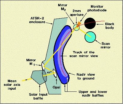
ATSR-2 (Along-Track Scanning Radiometer and Microwave Sounder-2)
The IRR instrument of ATSR-2 was upgraded for the ERS-2 mission by adding three more bands in the visible range to provide data for vegetation studies. The channels were accommodated by the addition of a second focal plane assembly (FPA). The centre wavelengths of the VIS channels were at 0.555, 0.659, and 0.865 µm (the IR channels are at 1.6, 3.7, 10.85 and 12 µm). The VIS channels were calibrated through a complex procedure using sunlight.21)
Major mechanical modifications were made to the ATSR-2 Infrared Radiometer (IRR). The carbon-fibre structure had been substantially re-designed, the vestigial ATSR-1 optical bench had been removed, and all-optical elements were mounted directly onto the structure.
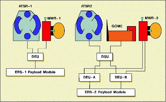
With the addition of GOME (Global Ozone Monitoring Experiment) for the ERS-2 mission, and the need to interface this experiment to the satellite via the ATSR-2's DEU (Digital Electronics Unit), it became important to add more redundancy to the latter as it interfaced with the IRR, the MWR and GOME. A second identical DEU was therefore added to the payload module, together with a DEU Switching Unit (DSU).
The visible channels were calibrated with a visible calibration unit, as shown in Figure 7. Calibration took place close to the time of local satellite sunset when the sun is 13º below the tangent to the Earth's surface at the satellite's nadir point. The nadir- and forward-viewing baffles were designed to exclude stray radiation from entering the calibration system, which would degrade its accuracy.
The increased data flow on ATSR-2 called for a new set of data compression algorithms. In addition, uncompressed infrared and visible data can be transmitted in a high-data-rate mode, which provides double the normal throughput. This mode is limited, however, to the periods when other payload instruments are not making full use of the X-band data capacity.
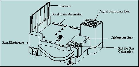
GOME (Global Ozone Monitoring Experiment)
GOME (also referred to as GOME-1) is an ESA-funded instrument developed and built by an industrial consortium in the time frame 1990-1994. The industrial consortium consisted of the Italian firms Officine Galileo and Laben (main electronics and electronic interface with ERS-2), British Aerospace (joint usage of the ATSR digital electronic interface), and the Dutch firm TPD (optical concept, calibration unit, pre-flight calibration). The German Remote Sensing Data Center (DFD) of DLR got the mandate to develop the GOME data processor system in collaboration with other institutes involved in the GOME Science Advisory Group.
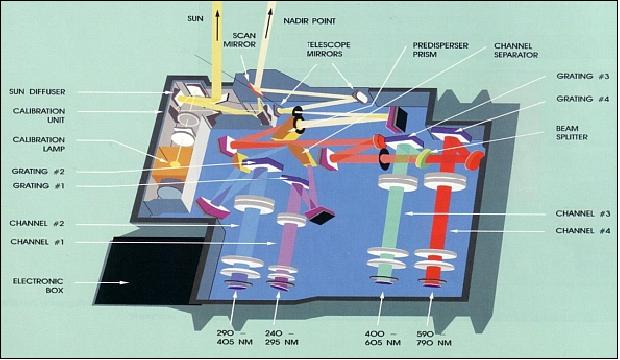
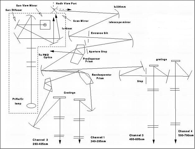
GOME is a cross-track scanning optical double spectrometer (or double monochromator), a nadir viewing instrument. The double spectrometer operates in the spectral range of 240 - 790 nm with a good spectral resolution of 0.2 - 0.4 nm; this decomposition is done in two steps: first by a quartz predisperser prism, from which the light is split into four different channels. Each of the four channels was equipped with a 1024-pixel linear diode array detector. The resulting spectral resolution was 0.2 nm in UV and 0.4 nm in the VNIR spectrum.
The goal of GOME was to observe upwelling solar radiation reflected or scattered in the Earth's atmosphere and from its surface. The measured spectrum contained absorption features which could be used to derive quantitative information on the presence of ozone and a number of other atmospheric species. In addition to the improved backscattering technique, GOME exploited the full capabilities of the enhanced ATSR-2. The GOME measurement concept was based on `Differential Optical Absorption Spectroscopy' (DOAS), a technology proven in balloon flights. 22) 23) 24) 25) 26) 27) 28) 29) 30) 31)
GOME science objectives:
Measurement of total column amounts and stratospheric and tropospheric profiles of ozone on a daily basis.
- In addition:
Measurement of column amounts of H2O and other gases involved in ozone photochemistry (like NO2, OClO, BrO, and possibly ClO in anticyclonic conditions, and pollutants like SO2 and HClO). GOME can also be used to investigate the distribution of atmospheric aerosols and clouds-plus-surface spectral reflectance.
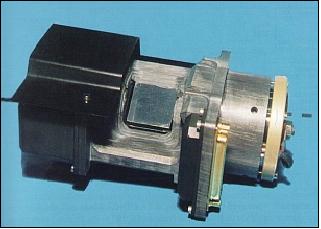
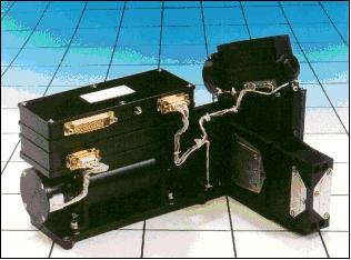
The GOME instrument consisted of the following functional modules:
- the spectrometer
- the four FPAs (Focal Plane Assembly)
- the calibration unit
- the scan electronics unit assembly
- the PMD (Polarization Measurement Device)
- the DDHU (Digital Data Handling Unit)
- the optical bench structure
- the thermal control unit.
Its main mode of operation was nadir-looking, but it was also able to look at the sun and the moon for calibration purposes. For onboard calibration, GOME did not depend on one technique but seeks to exploit several. Both absolute radiometric and wavelength calibrations were performed. This means that GOME retrieved ozone distributions by exploiting the traditional backscatter approach, as well as by the more novel differential optical absorption spectroscopy.
The IFOV (2.8º x 0.14º), corresponding to the projection of the spectrometer slit on the Earth, was a narrow rectangle of 40 km (along-track) x 2 km (across-track). A scan mirror sweeps the IFOV in the cross-track direction in three steps (normal mode), a ±31º scan (max). Maximum swath width = 960 km with corresponding pixel sizes of 40 km x 320 km. Smaller pixel sizes of 40 km x 40 km could be commanded (resulting in a smaller swath). With the 960 km swath global coverage could be achieved within three days.
Calibration was performed with regular views of the sun; in addition, a wavelength calibration lamp was used for wavelength stability. As the instrument was sensitive to the polarization of incoming radiation, a polarization detector monitors one polarization direction in the broadband channels corresponding essentially to detectors 2-4. GOME data rate = 40 kbit/s. GOME data were processed, archived and distributed at DLR/DFD.
GOME spectral bands:
- Channel 1A + 1B (237 -316 nm), 512 channels; [the Hartley bands of O3 and NO emission were the dominant features]
- Channel 2 (311 - 405 nm), 1024 channels; [a variety of target species absorbed in regions such as O3 (Huggin's band), O4, NO2, HCHO, SO2, BrO and OClO]
- Channel 3 (405 - 611 nm), 1024 channels; [the target molecules for this region were: NO2, OClO, O2, O3, (Chappius band), O4 and H2O]
- Channel 4 (595 - 793 nm), 1024 channels; [the target molecules were: O3 (Chappius band), NO3, H2O, and O2]
A combination of channels 2 to 4 could be used to make measurements of O2 and O4 column amounts (radiation penetration depths, cloud top heights).
Parameter | Value | Parameter | Value |
Spectral range | 240 - 790 nm | Spectral resolution | 0.2 - 0.4 nm |
Spatial resolution | 320 km x 40 km | No of spectral channels | 3500 |
Swath width | 120 - 960 km | Polarimetric channels | 3 |
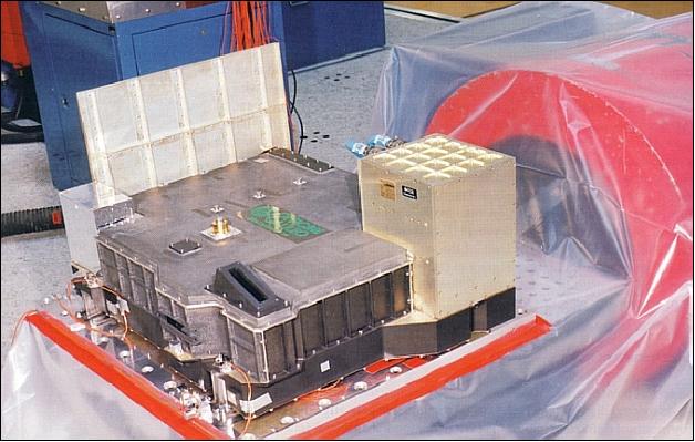
Calibration system | spectral lamp, | Instrument size | 60 cm x 70 cm x 50 cm |
Instrument mass | 50 kg | Power, bus voltage | 50 W, 22 V |
PRARE (Precise Range And Range-Rate Equipment) Tracking System
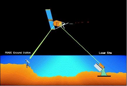
PRARE was a microwave tracking system operating at centimetre accuracy levels for the measurement of satellite-to-ground range and range rate. The concept was based on an autonomous spaceborne two-way and dual frequency microwave tracking system with its own:
a) telemetry,
b) telecommand,
c) data storage,
d) timing and data transmission capabilities.
This allowed data analysis on a global basis within a very short time delay. Due to the microwave transmission concept, the system operates independently from weather and daylight conditions.
Background:
The initial PRARE system development started in 1982 in Germany as a response to ESA's announcement of opportunity for exploitation of Europe's new Earth-remote sensing satellite series starting with ERS-1. The project was funded by BMFT and DARA, defined/designed by Ph. Hartl (University of Stuttgart) and Ch. Reigber of DGFI (German Geodetic Research Institute), Munich and since 1992 of GFZ (GeoForschungsZentrum), Potsdam. The space segment was built by Kayser Threde of Munich, and TimeTech GmbH of Stuttgart; the ground stations were developed by Dornier GmbH, Friedrichshafen. 32) 33) 34) 35) 36)
On ERS-1, the PRARE onboard instrument suffered a destructive RAM latch-up - resulting in a complete loss of the instrument operations about a week after the spacecraft launch. However, PRARE was successfully flown on the Russian mission Meteor-3-7 (launch: Jan. 25, 1994) as a passenger payload and a proof-of-concept mission for all PRARE subsystems. PRARE operations onboard Meteor-3-7 lasted for over a year providing excellent results; the operations were terminated in 1995 after the completion of all tests.
PRARE is also flown on ERS-2 (ESA procurement). It was in “operational status” as of Jan. 1, 1996 (i.e. the routine range and range rate product generation started on Jan. 1, 1996) providing measurement accuracies between 2.5 and 6.5 cm (two-way range data) and 0.1 mm/s (two-way range-rate data) respectively. PRARE operations were fully autonomous and separate from ERS-2 operations. 37) 38)
The PRARE system consisted of three major components
1) Space Segment:
This was a small self-contained hardware unit with a mass of 19 kg, power consumption of 39 VA (operational), or 8 VA in standby mode, and communication links independent of the host satellite.
2) Ground Station Network:
The network consisted of small automated and transportable ground stations (whose positions were known or could be determined from PRARE data to high precision). At X-band, a ground station worked as a regenerative and coherent transponder, at S-band a station acted as a receiver for the transmitted signals and measures the difference in the time of arrival of both signals.
3) Control Segment consisted of:
- GFZ's Master Station located at DLR in Oberpfaffenhofen, Germany
- TimeTech's Monitoring and System Command Station in Stuttgart, Germany
- A Calibration Station in Potsdam, Germany
These stations had special data evaluation, system control, and communication capabilities, which allowed them to fully control the space segment on ERS-2 as well as each individual ground station via the primary PRARE microwave links. This unique feature made the PRARE system operations independent from the host satellite (except for power) and adaptable for any near-Earth communication, navigation, or observation satellite system.
Applications:
The high-quality measurement of the PRARE data as well as their good global repeatability, density, and spatial distribution suited the data for deriving several higher-level geodynamic products for such applications as: 39)
- Precise satellite orbits
- Ground station coordinates
- Earth gravity field and Earth orientation parameters
- Ionospheric parameters
- Ultra-stable clock time information.
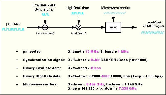
PRARE measurement principle:
Two continuous signals were emitted from the space segment to the ground, one of which is in the S-band (2.2 GHz), and the other in the X-band. Both signals were modulated with a PN-code (pseudo-random noise, 1 MChirp/s for the S-band and 10 MChirp/s for the X-band) used for the distance measurement and containing data signals (broadcast information) for ground station operation (prediction of orbit visibility, etc.). The time delay in the reception of the two simultaneously emitted signals was measured at the ground stations with an accuracy of better than 1 ns; the result is retransmitted and stored in the onboard memory of PRARE for later ionospheric correction of the data.
In the ground station the received X-band signal was transposed to 7.2 GHz, coherently modulated with the regenerated PN code (or with one of three orthogonal copies for code multiplexing) and including the two-frequency delay data as well as housekeeping and meteorological ground data was retransmitted to the PRARE space segment.
X-band uplink | - 7225.296 MHz (carrier frequency) |
Ground transponder power | 60 cm parabolic dish, 5 watts transmit |
X-band downlink | - 8489 MHz (carrier frequency) |
S-band downlink | - 248 MHz (carrier frequency) |
Satellite antennas | Crossed dipoles at X-band and S-band, 1 W in downlink and 5 W in uplink transmission power |
Noise values | ±1.5 cm rms for X-band ranging (1 measurement/s) |
Bias values | <1 cm for X-band; <3 cm for S-band (after post-processing) |
Range-error estimation | Tropospheric error: 2-7 cm; ionospheric error <1 cm; |
Total ranging accuracy | 2.5-6.5 cm (root squared sum) |
Total range-rate accuracy | 0.1 mm/s rms (root squared sum) |
The bandwidth-spread PRARE signals served simultaneously for the primary ranging purposes and for transmission of all necessary data among the system components. Both the user ground station network and the control segment could decode these superimposed data and reacted according to the information contained.
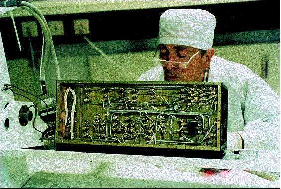
PRARE space segment
The PRARE space segment was developed and manufactured partly by the University of Stuttgart's Institute of Navigation (INS), and later by the private company TimeTech GmbH, Stuttgart. It consisted of a compact electronics box (dimensions 400 x 210 x 180 mm, power consumption 30 W in operational mode and 8 W in stand-by) and two crossed dipole antennas for transmission of the X-band and S-band signals. The X-band antenna also received the microwave signal after it has accomplished the round-trip transmission.
The space segment design featured four independent, parallel, strictly coherently operating receiver channels which tracked up to four PRARE ground stations that were in view of the satellite simultaneously. This allowed to generate an overlapping measurement data used for internal calibration and for back-up of the main orbit solution. This required a very careful internal hardware design and sophisticated control of all modules.
The very heart of the whole PRARE system was the internal oscillator of the space segment which was not only responsible for time tagging of the signal generation and communication processes but in fact controlled the complete system synchronization in ultra-short- (up to 1 second), in short- (up to 1000 seconds) and in long-term (more than 1000 seconds):
• Control of the internal coherency of the space segment signals, both for range and range-rate measurement data as well as for inter-channel coherency
• Time control of the whole ground station network by periodic synchronization pulse generation and transmission.
The PRARE space segment oscillator was an ultra-stable voltage-controlled quartz-crystal oscillator (VCXO) designed in the BVA technique and a state-of-the-art type of quartz oscillator. The primary output frequency was 5 MHz, which was divided/multiplied by the space segment electronics to generate all the frequencies necessary within the system.
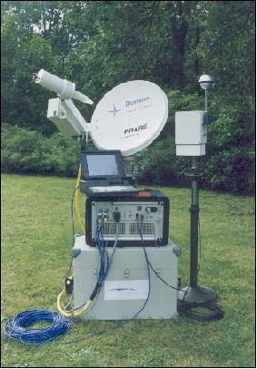
PRARE ground segment
Dedicated ground stations were used, which are acting basically as regenerative transponders.
A PRARE ground transponder consisted of:
- An antenna unit with an offset antenna of 60 cm diameter (parabolic dish), fronted electronics and tracking system. The antenna was fully movable in azimuth and elevation to track the satellite from horizon to horizon (weight 42 kg including gearing unit)
- An electronics unit including RF-modules (dimensions 560 x 560 x 300 mm, weight 35 kg), linked together by RF-signal and data cables. The electronic tracking loops filter the received microwave signal, decode the superimposed data (low-rate modulation), which contained dedicated information for each individual ground station, transpose the microwave frequency to the uplink (fixed frequency ratio 749/880), re-modulate new site-specific low-rate information, and send the signal back to the satellite.
The PRARE ground station tracking network consisted of 29 PRARE transponders in total (globally distributed), which are owned by 10 different international geodetic research groups (plus GFZ) and operated locally by co-operating scientific institutions.
During satellite contact, the main tasks of the ground station modules were:
- X-band signal transponding
- Measurement of the delay difference between the quasi-simultaneously transmitted S- and X-band signals
- Measurement of the internal X-/X-signal path delay
- Meteorological data handling, acquired at the ground station site
- Clock pulse and time generation and synchronization
- Low-rate and high-rate data reception and interpretation
- Low-rate data transmission
- Setup and calibration of data interpretation and storage.
ERS Tandem Mission (Oct. 1995 to June 1996)
In 1993, the ERS science community realized that a future tandem mission of the healthy ERS-1 spacecraft and a planned launch of the ERS-2 satellite in 1995 would be a great possibility for interferometric experimentation in SAR observations. As a consequence, the ESA Council adopted a resolution in March 1995 - with the objective to provide ERS-1/2 tandem mission operations for a nominal period of 9 months (starting with the ERS-2 operational phase) and to keep ERS-1 operational for at least until April 1997. 40) 41) 42)
In the orbital tandem, the configuration of both spacecraft in the same orbit, ERS-2 follows ERS-1 with an approximate delay (referred to as orbit phasing) of 35 minutes. The configuration was that of two-pass measurements of a single-antenna SAR platform (the same SAR instrument on both satellites observing the same area on the ground), permitting the superposition technique of imagery (in data processing) of fairly close repeat tracks.
Due to the phasing and the Earth's rotation, the ground-track patterns of ERS-2 are slightly shifted westwards with respect to those of ERS-1. The orbit phasing is adjusted in such a way that the ERS-2 track coincides exactly with that of ERS-1, however 24 hours earlier.
The benefits of tandem operations were the following:
• When the same area of the Earth was observed by the same instrument on both satellites with a ground-site revisiting interval of 1 or 8 days, the improvements compared to a single satellite were:
- the number of acquisitions in a repeat cycle (35 days) was doubled
- the time interval between two successive acquisitions was shorter, being 1 to 8 days rather than 35 days
• For global applications, such as wind scatterometer data, coverage was doubled within a given time period
• When the ground-track pattern of nadir-looking instruments on one satellite overlap the ground tracks of side-looking instruments on the other satellite, then their information can be combined, providing synergistic benefits.
The greatest benefit of the tandem mission was seen in SAR interferometry providing excellent temporal (1-day interval) and spatial coherence. This technique required two separate images taken of the same ground track by two spatially-separated antennas (the interferometric baseline) to produce phase differences from slightly different viewing angles. For each pixel corresponding to the same area of the ground in both images, the phase values (depending on the satellite-to-ground pixel length) were subtracted to produce a phase difference image known as the `interferogram.' With the orbit of both satellites known, the phase interferogram could be used to generate a DEM (Digital Elevation Model) of the surface with an accuracy of about 10 m.
An additional product of interferometry was the so-called `coherence image,' which showed bright areas where the coherence between to SAR images is high, indicating no variation in backscatter between the acquisition times of the two images. Dark regions indicated areas where changes had occurred.
ERS-1 and ERS-2 have been in tandem operations since about September 1995. The tandem mission was completed after nine months of successful operation in May/June 1996. About 110,000 ERS SAR pairs of data were acquired during the tandem mission, covering nearly the whole global land surface. Over South America and part of Southeast Asia, just one data pair was acquired. As many as five or six interferometric pairs were available for Europe and North America, allowing greater accuracies to be achieved. 43) 44)
The ERS Tandem Mission encompassed the following combinations of instrument data:
• The same instrument on both satellites observing the same area on the ground with a one-day interval, e.g. for SAR interferometry and/or change detection. ERS SAR interferometry had already been validated using ERS-1 data only, with a 3 or 35-day repeat cycle. The one-day offset offered by the tandem mission increased the probability of having high coherence between the acquired data
• The same instrument on both satellites observing different areas on the ground on the same day, to provide increased spatial sampling
• Different instruments observing the same areas on the ground with a very short interval (less than 1 hr), e.g. the AMI-SCAT (wind scatterometer mode) and the Radar Altimeter for comparison of wind measurements.
The ERS tandem mission generated a large resource of interferometric SAR data (InSAR) for analysis in the geosciences.
Nominal observation services of each mission (ERS-1 and -2) commenced after completion of the tandem mission in June 1996.
References
1) C. R. Francis, G. Graf, P. G. Edwards, M. McCaig, C. McCarthy, A. Lefebvre, B. Pieper, et al., “The ERS-2 Spacecraft and its Payload,” ESA Bulletin, No. 83, Aug. 1995, pp. 13-31,
2) G. Duchossois, P. Martin, “ERS-1 and ERS-2 Tandem Operations,” ESA Bulletin, No. 83, August 1995, pp. 54-60
3) “ERS satellite missions complete after 20 years,” ESA, Sept. 12, 2011, URL: http://www.esa.int/esaCP/SEM8Q40UDSG_index_0.html
4) “Pioneering ERS environment satellite retires,” ESA, July 5, 2011, URL: http://www.esa.int/esaEO/SEMJ0O6TLPG_index_0.html
5) “ERS-2 status,” ESA Bulletin, No 145, Feb. 2011, p. 81
6) “Last 'tango' in space,” ESA, Nov. 2, 2010, URL: http://www.esa.int/esaEO/SEMSSJ4PVFG_index_0.html
7) “ERS-2 Satellite Celebrates 15th Anniversary,” April 21, 2010, URL: http://www.redorbit.com/news/space/1853256/ers2_satellite_celebrates_15th_anniversary/
8) http://earth.esa.int/ers/technicalstatusreport/
10) http://www.esa.int/esaMI/Operations/SEMM1Z8L6VE_0.html
11) Henri Laur, “SAR Interferometry opportunities with the European Space Agency: ERS-1, ERS-2, Envisat, Sentinel-1A, Sentinel-1B, ESA 3rdParty Missions (ALOS),” Fringe 2009 Workshop - Advances in the Science and Applications of SAR Interferometry, Frascati, Italy, Nov. 30-Dec. 4, 2009, URL: http://earth.esa.int/workshops/fringe09/participants/758/pres_758_HLaur.pdf
12) “ESA satellites flying in formation,” Dec. 3, 2008, URL: http://www.esa.int/esaEO/SEMWI74Z2OF_index_0.html
13) M. A. Martín Serrano, M. A. García Matatoros, M. E. Engdahl, “Achieving the ERS-2 - Envisat inter-satellite interferometry tandem constellation,” URL: http://www.mediatec-dif.com/issfd/OperaI/Martin%20Serrano.pdf
14) “ESA's old EO missions perform sophisticated new tricks,” April 29, 2009, URL: http://news.eoportal.org/eomissions/090505_eom2.html
15) The information was provided by Franz-Heinrich Massmann of GFZ (GeoForschungszentrum), Berlin, Germany
16) N. Miranda, B. Risich, C. Santella, M. Grion, “Review of the Impact of the ERS-2 Piloting Modes on the SAR Doppler Stability,” Envisat and ERS Symposium, Salzburg, Austria, Sept. 6-10, 2004, ESA publication SP-572
17) W. Lengert, “ERS missions overview,” Fringe Workshop 2003, ESA/ESRIN, Frascati, Italy, Dec. 1-5, 2003
18) Project News, ERS, ESA Earth Observation Quarterly No 69, p.4, June 2001
19) Project News, ERS, ESA Earth Observation Quarterly No 70, p.4, January 2002
20) X. Neyt, P. Pettiaux, M. Acheroy, “Scatterometer Ground Processing Review for Gyro¿Less Operations,” Proceedings of SPIE, Vol. 4881, 9th International Symposium on Remote Sensing, Aghia Pelagia, Crete, Greece, Sept. 23¿27, 2002
21) N. Stricker, A. Hahne, D. L. Smith, J. Delderfield, M. B. Oliver, T. Edwards, “ATSR-2: The Evolution in its Design from ERS-1 to ERS-2,” ESA Bulletin No. 83, August 1995, pp. 32-37
22) ESA 1998: GOME Special, Earth Observation Quarterly No. 58, March 1998
23) “The GOME Spectrometer,” URL: http://www.iup.uni-bremen.de/gome/gomeinst.html
24) C. Zehner, G. Pittella, “Preparing atmospheric applications for future ESA Earth-observation missions in the frame of the data user program, ESA Earth Observation Quarterly No. 61, Feb. 1999, pp. 1-6
25) C.J. Readings, `The Interim GOME Science Report,' Feb. 1990,
26) `The Global Ozone Monitoring Experiment (GOME) and ERS-2,' Earth Observation Quarterly, ESA periodical No. 32 Dec. 1990
27) A. Hahne, et al., “GOME: A New Instrument for ERS-2,” ESA Bulletin, No. 73, February 1993, pp. 22-29
28) GOME Global Ozone Monitoring Experiment, Interim Science Report, ESA SP-1151, September 1993
29) J. P. Burrows, M. Weber, M. Eisinger, “The Global Ozone Monitoring Experiment - GOME,” SPARC Newsletter 09, July1997
30) J. P. Burrows, M. Weber, M. Buchwitz, V. Rozanov, A. Ladstätter-Weissenmayer, A. Richter, R. DeBeek,R. Hoogen, K. Bramstedt, K.-U. Eichmann, M. Eisinger, D. Perner, “The Global Ozone Monitoring Experiment (GOME): Mission concept and first scientific results,” Journal of Atmospheric Science, Vol 56, January 15, 1999, pp. 151-175 , URL: http://www.iup.uni-bremen.de/UVSAT_material/papers/Burrows_JAS1999.pdf
31)) A. Hahne, A. Lefebvre, J. Callies, B. Christensen, “GOME - The Development of a New Instrument,” ESA Bulletin No. 83, August 1995
32) P. Hartl, C. Reigber, “Das PRARE-System der ERS-1 Mission,” Geowissenschaften Vol. 9, No. 4/5, 1991, pp. 156-162
33) P. Hartl, C. Reigber, “Das Satellitenbeobachtungssystem PRARE. Zeitschrift für Vermessungswesen, Vol. 12, 1990, pp. 512-519
34) F. Flechtner, K. Kaniuth, Ch. Reigber, H. Wilmes, “The Precise Range and Range Rate Equipment PRARE: Status Report on System Development, Preparations for ERS-1 and Future Plans,” Second International Symposium on Precise Positioning with the Global Positioning System (GPS '90), Sept. `90, Ottawa, Canada
35) P. Hartl, C. Reigber “Das PRARE-System der ERS-1 Mission,” Die Geowissenschaften, 9. Jahrgang, Heft 4-5, April-Mei 1991, pp. 156-162.
36) W. Schäfer, W. Schumann, “PRARE-2 - Building on the Lessons Learnt from ERS-1,” ESA Bulletin No 83, August 1995
37) Ch. Reigber, F.-H. Massmann, F. Flechtner, “The PRARE System and the Data Analysis Procedure,” CSTG Bulletin Vol. 14, 1997, pp. 11-19
38) F.-H. >Massmann, F. Flechtner, J.-C. Raimondo, C. Reigber, “Impact of PRARE on ERS-2 POD,” Advances in Space Research, Vol. 19, No 11, 1997, pp. 1645-1648
39) P. N. A. M Visser, R. Scharroo, R. Floberghagen, B. A .C. Ambrosius, “Impact of PRARE on ERS-2 orbit determination.,” Proceedings of the 12th International Symposium on Space Flight Dynamics, ESA-SP403, pp. 115-120, 1997
40)) G. Duchossois, P. Martin, “ERS-1 and ERS-2 Tandem Operations,” ESA Bulletin No 83, Aug. 1995
41) G. Duchossois, G. Kohlhammer, P. Martin, “Completion of the ERS Tandem Mission,” ESA Earth Observation Quarterly, June 1996
42) J. M. Dow, M. Rosengren, X. Marc, R. Zandbergen, R. Piriz, M. Romay Merino, “Achieving, Assessing and Exploiting the ERS-1/2 Tandem Orbit Configuration,” ESA Bulletin, No 85, February 1996
43) “Case Study 16: SAR Interferometry,” pp. 107-115, in `Further Achievements of the ERS Missions,' ESA SP-1228, Dec. 1998, ISBN: 92-9092-508-6
44) L. Timmen, X. Ye, C. Reigber, R. Hartmann, T. Fiksel, W. Winzer, J. Knoch-Weber, “Monitoring of Small Motions in Mining Areas by SAR Interferometry,” Proceedings of FRINGE 96, ERS SAR Interferometry Workshop 1996, University of Zürich, Switzerland, Sept. 30, Oct. 2, 1996
45) ESA, “ESA’s ERS-2 satellite will reenter Earth’s atmosphere in February 2024”, February 5, 2024, URL: https://blogs.esa.int/rocketscience/2024/02/05/ers-2-reentry-homepage/
46) ESA, “ERS-2 reenters Earth’s atmosphere over Pacific Ocean”, February 21, 2024, URL: https://www.esa.int/Space_Safety/Space_Debris/ERS-2_reenters_Earth_s_atmosphere_over_Pacific_Ocean