Landsat-8 - 2017 to 2013
Landsat-8 Imagery in the period 2017 to June 2013
2017 2016 2015 2014 2013 References
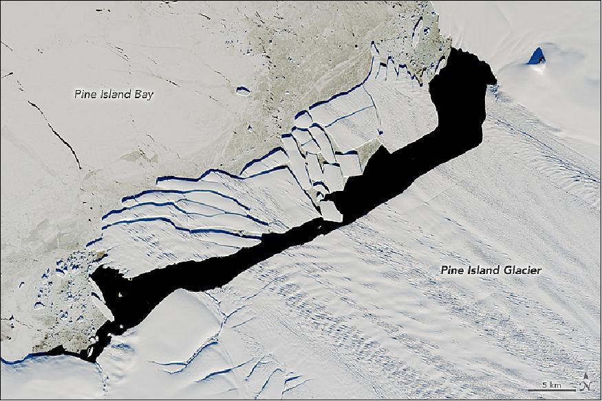
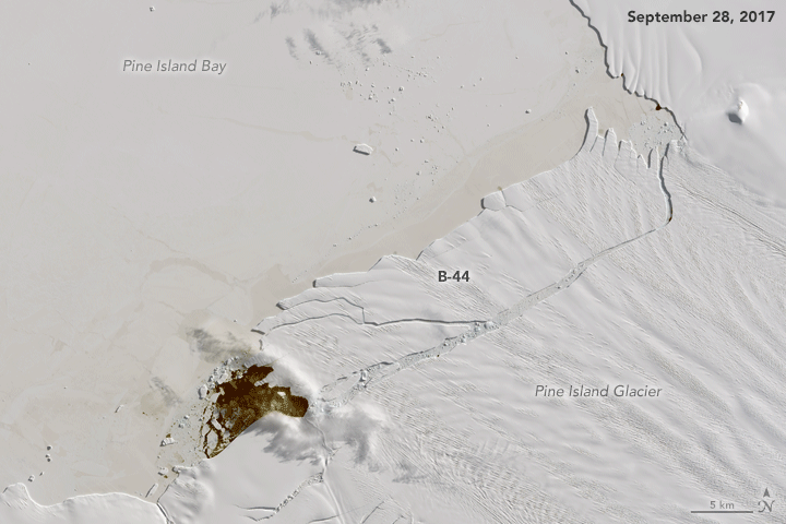
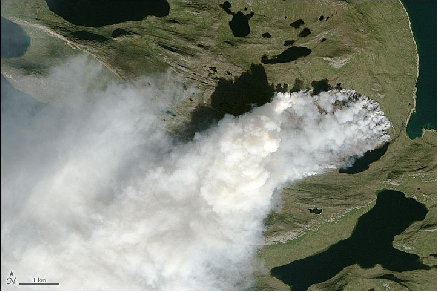
• December 26, 2017: In September 2017, a new iceberg calved from Pine Island Glacier—one of the main outlets where the West Antarctic Ice Sheet flows into the ocean. Just weeks later, the berg named B-44 shattered into more than 20 fragments. 1)
- On December 15, 2017, OLI (Operational Land Imager) on Landsat-8 acquired a natural-color image (Figure 1) of the broken iceberg. An area of relatively warm water, known as a polyna, has kept the water ice free between the iceberg chunks and the glacier front. NASA glaciologist Chris Shuman thinks the polynya's warm water could have caused the rapid breakup of B-44.
- The image of Figure 1 was acquired near midnight local time. Based on parameters including the azimuth of the Sun and its elevation above the horizon, as well as the length of the shadows, Shuman has estimated that the iceberg rises about 49 meters above the water line. That would put the total thickness of the berg—above and below the water surface—at about 315 meters.
• December 24, 2017: Before the opening of the Panama Canal in 1914, Cape Horn was a place that gave mariners nightmares. The waters off this rocky point, at the southern tip of Chile's Tierra del Fuego peninsula, pose a perfect storm of hazards. 2)
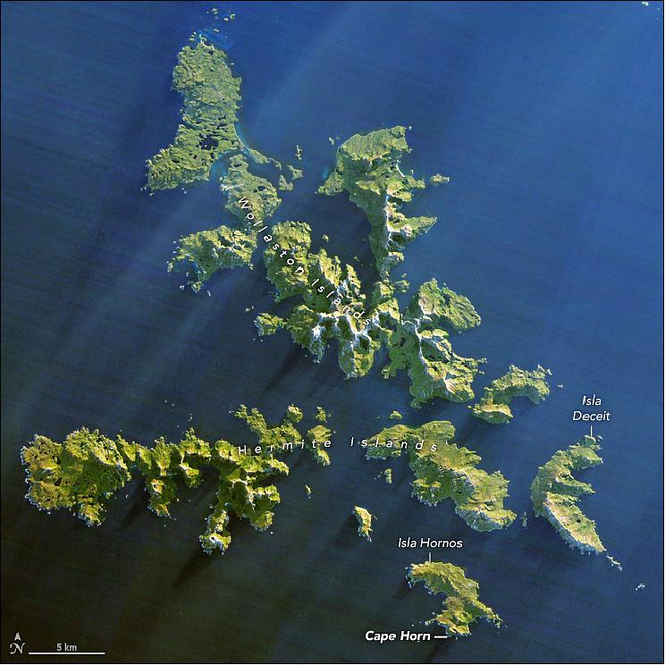
- Southwest of Cape Horn, the ocean floor rises sharply from 4,020 m to 100 m within a few kilometers. This sharp difference, combined with the potent westerly winds that swirl around the Furious Fifties, pushes up massive waves with frightening regularity. Add in frigid water temperatures, rocky coastal shoals, and stray icebergs—which drift north from Antarctica across the Drake Passage—and it is easy to see why the area is known as a graveyard for ships.
- Hundreds of ships have gone down near Cape Horn since Dutchman Willem Schouten, a navigator for the Dutch East India Company, first charted a course around the Horn in 1616. One vessel that narrowly escaped that fate was the HMS Beagle, with naturalist Charles Darwin aboard. In 'The Voyage of the Beagle', Darwin described the harrowing journey as the explorers tried to round the Horn just before Christmas 1832.
December 21st. — The Beagle got under way: and on the succeeding day, favored to an uncommon degree by a fine easterly breeze, we closed in with the Barnevelts, and running past Cape Deceit with its stony peaks, about three o'clock doubled the weather-beaten Cape Horn. The evening was calm and bright, and we enjoyed a fine view of the surrounding isles. Cape Horn, however, demanded his tribute, and before night sent us a gale of wind directly in our teeth. We stood out to sea, and on the second day again made the land, when we saw on our weather-bow this notorious promontory in its proper form—veiled in a mist, and its dim outline surrounded by a storm of wind and water. Great black clouds were rolling across the heavens, and squalls of rain, with hail, swept by us with such extreme violence, that the Captain determined to run into Wigwam Cove. This is a snug little harbor, not far from Cape Horn; and here, at Christmas-eve, we anchored in smooth water. The only thing which reminded us of the gale outside, was every now and then a puff from the mountains, which made the ship surge at her anchors. |
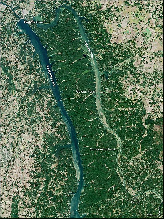
• December 15, 2017: For more than a hundred years, the fertile and forested patch between the Tennessee and Cumberland rivers was referred to as the "land between the rivers." In the 1960s, it became the "land between the lakes." 3)
- In an attempt to control flooding and to generate electricity in rural Kentucky and Tennessee, the TVA (Tennessee Valley Authority) built Kentucky Dam, thereby impounding the Tennessee River and creating Kentucky Lake in 1944. It became the largest manmade lake east of the Mississippi River.
- Two decades later, the U.S. Army Corps of Engineers blocked the flow of the nearby Cumberland River as well. With the completion of Barkley Dam in 1966, the waters of the Cumberland piled up into Lake Barkley. In the process of creating the two lakes, residents of several small towns along and between the rivers were moved, and parts of some towns were permanently flooded. A few local roads and railways had to be re-routed.
- Engineers also dug out Barkley Canal in order to bring the two rivers and lakes to the same water level. This allowed ships and barges to more easily move goods (without locks) from the Cumberland and Tennessee river valleys toward the mighty Mississippi River. By the time they were done, the TVA and Army Corps had created one of the largest inland peninsulas in the United States.
- In the years after the lakes were created, the new peninsula was slowly converted into a recreation area for hunting, fishing, boating, hiking, and camping. Now managed by the U.S. Forest Service, the Land Between the Lakes National Recreation Area includes one of the largest freshwater recreation complexes in the United States. The parkland and lakes attract roughly two million visitors per year. The Operational Land Imager (OLI) on Landsat 8 acquired this natural-color image of the region on October 7, 2016.
- Near Golden Pond, some forests have been cleared and re-seeded to return the land to what it likely looked in the 19th century. That grassland prairie also has been settled with elk and bison that once roamed the region. Recreational facilities also include a planetarium and a woodlands nature station. At the southern end of Land Between the Lakes, near the town of Dover, a re-creation of an 1850s homestead includes rare breeds of livestock and plants from that era.
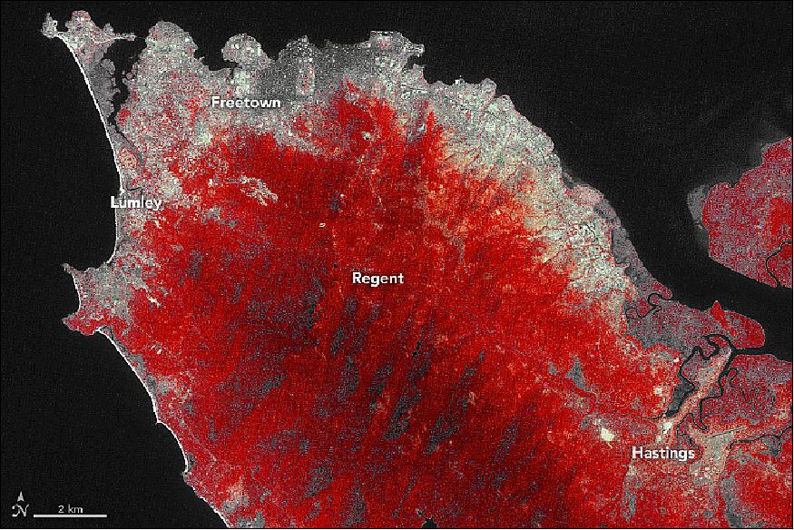
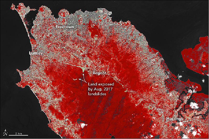
• December 5, 2017: At 6:50 a.m. on August 14, 2017, the people of Regent heard a low rumbling noise like the hum of a passing airplane. Then there was quiet. A hillside had failed in this mountainous area just beyond Freetown, Sierra Leone (Africa, located on the Atlantic Ocean). 4)
- Ten minutes later, an explosive sound came from the direction of nearby Mount Sugar Loaf. The Earth trembled and began to flow. Trees and boulders of all sizes tumbled chaotically. Sparks lit the morning air as metal and rock collided. A river of rust-colored soil plunged into the swollen stream valleys below, which were already filled with floodwater due to several days of intense rain. A destructive slurry of mud, boulders, and tree parts rushed down toward the stream valley, flowing more than three kilometers before draining into the sea near Lumley.
- When authorities tallied the loss of life and property, the numbers were sobering. More than 1,141 people died and 3,000 people lost their homes, according to a World Bank assessment. Damage to homes in the area totaled more than $14 million.
- Sustained downpours were the immediate trigger for the landslide. Between July 1 and August 14, Freetown received 1,040 mm of rain—about three times the norm for that period. However, decades of rapid urbanization in landslide-prone areas, as well as construction along streams where flooding was common, set the stage for the disaster. Joseph McCarthy, an urban planner at Njala University, went so far as to tell Thompson Reuters that: "The major cause of mudslides and flooding is the chaotic development caused by the rapid urbanization of Freetown."
- This pair of false-color Landsat images (Figures 5 and 6) illustrates the extent of the changes. Forested areas appear red, urban areas are gray, and landslide debris is tan. In 1986, most of the development was in low-lying, coastal areas. By 2017, development had spread widely into mountainous areas. For instance, the town of Regent had just a handful of buildings in 1986. By 2017, it had many more buildings and a population of 28,000 people.
- In addition to the spread of urban areas, the images also highlight the extent of deforestation—one of the factors that helps trigger landslides—to the south of Freetown. According to one analysis of Landsat imagery led by Lamin Mansaray of Zhejiang University, the Freetown region saw its densely forested areas drop from 113 km2 in 1986 to 59 km2 in 2015 — a 52 percent decline.
- The city's population increased from about 500,000 people in 1986 to about 1 million people today. A civil war between 1991–2002 accelerated the city's expansion. "Before 1991, there was minimal rural-urban migration in Sierra Leone. During the conflict, rural areas were most vulnerable to attacks, and Freetown was by far the safest place to be," explained Mansaray. "After the war ended in 2002, migration into the capital remained high because most people in rural areas had lost their homes and sources of livelihoods."
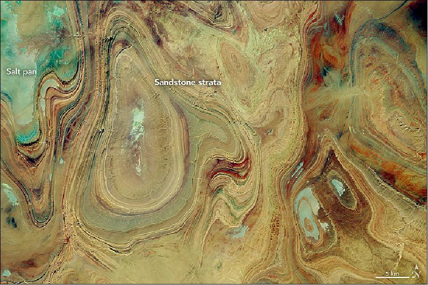
• December 2, 2017: In central Algeria, just above the Tropic of Cancer and about 1200 km south of the Algiers metropolis, lies a land as desolate as it is beautiful. 5)
- In this part of the Sahara, known as the Tanezrouft Basin, the land is especially parched, with annual rainfall measured in mm (less than 5 mm). This is a hyperarid place of soaring temperatures and scarce access to water or vegetation. There are no permanent residents here, only occasional Tuareg nomads. The basin's colloquial name is the "Land of Terror" because, for many, to traverse this land is to stare death in the face.
- The severe conditions that make this basin a barren expanse for life also lay bare its exquisite geology. Wind erosion—caused by constant sandblasting through millennia of frequent sandstorms—has exposed ancient folds in the Paleozoic rocks. This natural-color image, acquired on October 22, 2017, by OLI (Operational Land Imager) on Landsat 8, shows concentric rings of exposed sandstone strata that create stunning patterns across the Tanezrouft Basin. When viewed from 705 km above Earth, the exposed geologic features create an arresting work of abstract art.
- The sandstone canyons in this region have walls that rise as high as 500 m, and salt flats can be found in their lower reaches. The flats indicate that water played a role in sculpting this landscape. "Intermittent flooding has occurred often enough to mold the landscape pretty thoroughly over millions of years," explained P. Kyle House, a geologist with the U.S. Geological Survey. "There are numerous canyons in this region that both follow and abruptly cut directly across the grain of the tilted and folded strata," he added. "These patterns are striking and reminiscent of landscapes formed on folded strata in, for example, the Red Desert of southern Wyoming and even parts of the heavily forested Appalachian Mountains of the Eastern United States."
- On the ground, life is a rare. About 80 km east of this area, the trans-Saharan highway—known as one of the world's most brutal roads—makes its way through the desert.
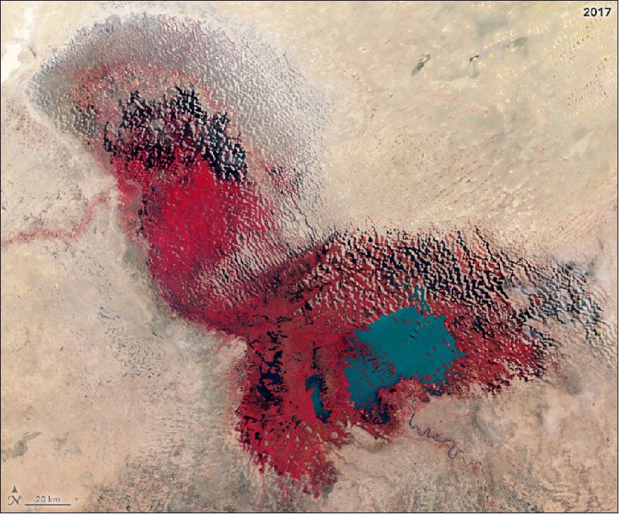
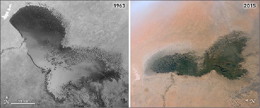
• November 25, 2017: Lake Chad sustains people, animals, fishing, irrigation, and economic activity in west-central Africa. But in the past half century, the once-great lake has lost most of its water and now spans less than a tenth of the area it covered in the 1960s. Scientists and resource managers are concerned about the dramatic loss of fresh water that is the lifeblood of more than 30 million people. 6) 7)
- Lake Chad sits within the Sahel, a semiarid strip of land dividing the Sahara Desert from the humid savannas of equatorial Africa. The Chad Basin is bordered by mountain ranges and spans more than 2.4 million km2 of Cameroon, Nigeria, Chad, and Niger. The water level is largely controlled by the inflow from rivers, notably the Chari River from the south and, seasonally, the Komodugu-Yobe from the northwest. Rainfall can also reach the lake by way of smaller tributaries and groundwater discharge.
- Inflow fluctuates with the shifting patterns of rainfall associated with the West African Monsoon, making the system very sensitive to drought. Most precipitation in the Sahel falls during the peak of a short rainy season from July through September. The dry season is most intense between November and March. Years with little precipitation can wreak havoc on the water supply.
- Extreme swings in Lake Chad's water levels are not new. The lake has experienced wet and dry periods for thousands of years, according to paleoclimate research. More recently, variations in depth and extent were noted by French explorer Jean Tilho, who reported in 1910 that parts of the lake had dried up. But what is new is the way researchers are studying changes in the lake.
- The images of Figures 8 to 10 highlight the shrinking and growing in the recent life of Lake Chad. The false-color images were acquired by Landsat satellites—Landsat-1 in 1973 and Landsat-8 in 2017. The combination of visible and infrared light helps to better differentiate between vegetation (red) and water (blue and slate gray). The photographs of Figure 10 were captured by the Corona reconnaissance satellite in 1963 and by an astronaut on the International Space Station in 2015.
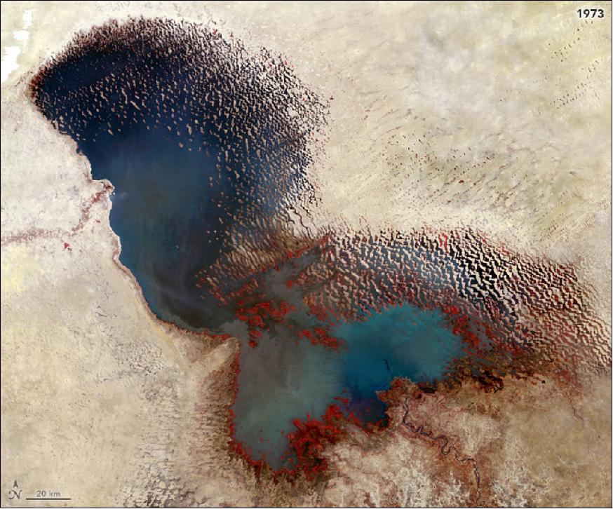
- In 1973, the lake was in a phase called "Normal Lake Chad"—a single body of water with an archipelago on the north side of the southern basin. Note how little vegetation was around the lake at that stage. Throughout the 1970s, severe droughts plagued the African Sahel, and water disappeared from the northern basin. Since then, water has come and gone from the northern lobe depending on the year and season. But the two lobes have never reconnected into a single lake.
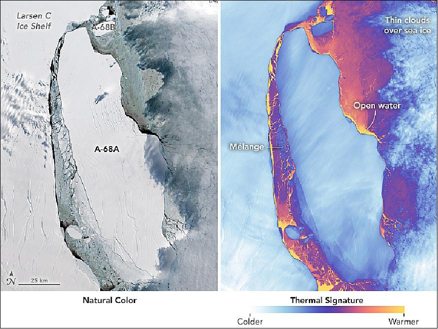
• November 2017: A lot happened on the Antarctic Peninsula under the cloak of the 2017 polar night—most notably, the calving of a massive iceberg from the Larsen C ice shelf. At the time (July), scientists had to rely on thermal imagery and radar data to observe the break and to watch the subsequent motion of the ice. 8) 9)
- By August, scientists started getting their first sunlit views of the new iceberg, which the U.S. National Ice Center named A-68. MODIS (Moderate Resolution Imaging Spectroradiometer) on NASA's Terra satellite captured a wide view of the berg on September 11. A few days later, on September 16, the OLI (Operational Land Imager) and TIRS (Thermal Infrared Sensor) on Landsat-8 captured these detailed images.
- The image on the left of Figure 11 shows the icebergs in natural color. The rifts on the main berg and ice shelf stand out, while clouds on the east side cast a shadow on the berg. The thermal image on the right shows the same area in false-color. Note that the clouds over the ice shelf do not show up as well in the thermal image because they are about the same temperature as the shelf. Thermal imagery has the advantage of showing where the colder ice ends and "warm" water of the Weddell Sea begins. It also indicates differences in the thickness of ice types. For example, the mélange is thicker (has a colder signal) than the frazil ice, but thinner (warmer signal) than the shelf and icebergs.
- Both images show a thin layer of frazil ice, which does not offer much resistance as winds, tides, and currents try to move the massive iceberg away from the Larsen C ice shelf. In a few weeks of observations, scientists have seen the passage widen between the main iceberg and the front of the shelf. This slow widening comes after an initial back-and-forth movement in July broke the main berg into two large pieces, which the U.S. National Ice Center named A-68A and A-68B. The collisions also produced a handful of pieces too small to be named.
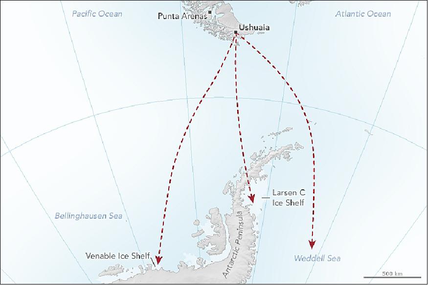
• November 11, 2017: Ushuaia, Argentina, is many things to the growing number of people who live there: the southernmost city in the world, the gateway to Antarctica, and a gorgeous home along a rocky coast. For NASA, the city's southerly location makes it an ideal place to stage science flights to Antarctica. 10)
- The flights are part of Operation IceBridge, NASA's longest-running mission to map polar ice (now in its ninth year in the Southern Hemisphere). For the first time, flights over the icy continent are being staged from Ushuaia, instead of Punta Arenas, Chile. Read more about this campaign on our blog.
- OLI (Operational Land Imager) on Landsat-8 captured this image of Ushuaia on March 28, 2017. Located at the tip of South America, it is the capital city of Tierra del Fuego province. Port Williams lies across the channel from Ushuaia, but the village is too small to be visible in this natural-color image.
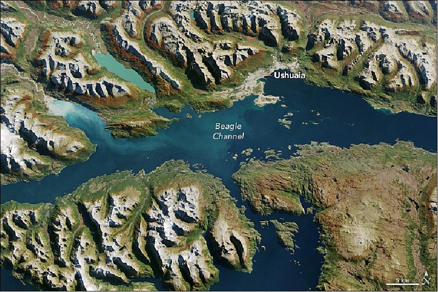
- Ushuaia is located about 250 km southeast of Punta Arenas, Chile. The city's proximity to the Antarctic Peninsula means that NASA's IceBridge campaign scientists gain an hour of extra flight time over science targets. That's important because the P-3 aircraft being flown during this campaign has a shorter range than the DC-8 aircraft flown during previous campaigns. The map of Figure 13 represents how flights from Ushuaia might cross the Southern Ocean to observe the Antarctic Peninsula and its surrounding seas and ice.
- Science flights began on October 29, and the spring weather in Ushuaia has been relatively mild for the first few weeks of the campaign. But as the locals say, you can get four seasons in any given day here. Strong winds, cold temperatures, and heavy rain are not out of the question. Living or visiting here means you should be ready for any kind of weather at all times.
- The extent of the urban area visible in the satellite image shows that, indeed, the city covers a sizeable area for such a remote part of the world (23 km2). Census information from 2010 reported the population in Ushuaia to be 56,956—almost double the population in 1991. Still, that's just a small fraction of the country's total population of more than 40 million people, most of whom live in Buenos Aires province.
- Ushuaia's port is partially used for industry; container ships dock here, and cargo boxes are stacked in tidy, colorful rows along the shore. Tourism is also important: People come from around the world to hike in Tierra del Fuego National Park, ski in the mountains, cruise to see penguins on Martillo Island, or catch a cruise ship to Antarctica.
Improvements to the quality and usability of Landsat satellite data have been made with the release of a new USGS product called Landsat Analysis Ready Data (ARD). This product will help reduce the time needed to process and analyze data and imagery, a significant advantage to scientists studying landscape changes, including changes from wildfires, hurricanes, vegetation cover, drought and other events. A fundamental goal for Landsat ARD is to significantly reduce the amount of data processing for scientists, who currently have to download and prepare large amounts of Landsat scene-based data for time-series investigative analysis. ARD provides users with notable flexibility in how they access customized Landsat data. For example, users will have the ability to tailor requests according to specific needs in terms of geospatial regions, spectral bands and collection dates. Landsat data are the world's longest continuously acquired collection of space-based land remote sensing data. ARD products represent over 30 years of Landsat data available at the highest scientific quality ever produced. This initial ARD release includes Landsat 4-8 imagery of the conterminous United States, Alaska and Hawaii. In the future, the USGS plans to add the earlier Landsat 1-5 Multispectral Scanner era imagery to the ARD product suite and eventually expand ARD to include the full global Landsat archive. ARD will serve many purposes such as the foundational dataset for the recent USGS Land Change Monitoring, Assessment, and Projection (LCMAP) initiative. The initiative aims to characterize historical and near-real time land-cover changes across the United States. The ARD products are based on the recently released Landsat Level-1 Collection structure. Landsat Level-1 products refer to the most basic level of processing that has been applied to a scene for them to be used in applications. This collection management structure ensures access to Landsat Level-1 products as they are acquired and a consistent archive of known data quality. The USGS generates ARD products from data acquired by the Landsat 4-5 Thematic Mapper, Landsat 7 Enhanced Thematic Mapper Plus and Landsat 8 Operational Land Imager and Thermal Infrared Sensor instruments. Landsat ARD is created after processing Landsat Level-1 Collection scenes into Albers Equal Area Conic projection. The USGS processes these products to create top of atmosphere reflectance, brightness temperature and atmospherically corrected surface reflectance. The USGS assembles these products into "tiles" adapted from the Web Enabled Landsat Data tiling scheme. This tiling scheme ensures that each pixel in an ARD tile represents the same location on the Earth's surface through the entire ARD time series record from 1982 to the present. In addition to this higher-level spectral band processing of geophysical parameters, ARD includes several pixel-level quality assessment bands. These bands document the presence of sensor, solar, atmospheric and topographic conditions and traceability to the Landsat Level-1 input source scenes used in ARD. Each ARD tile product is accompanied by comprehensive metadata that ensures full traceability to the Level-1 input source scenes as well as the versions of the algorithms and processing software used to generate them. The USGS has documented ARD product characteristics in the Landsat ARD Data Format Control Book. ARD results from a USGS-NASA decision to make Landsat data more relevant for the next generation of information applications. -Users can access Landsat ARD through the EarthExplorer data portal. |
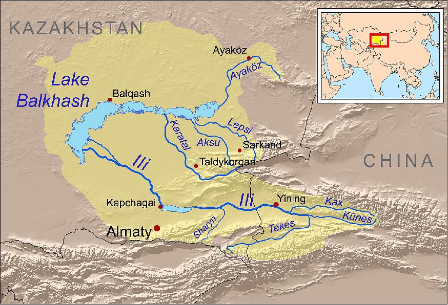
• November 4, 2017: The Aral Sea and Lake Balkhash have a lot in common. Both lakes are located in an arid part of Central Asia; both are somewhat saline; and neither has an outlet. But after the desiccation of the Aral Sea—once the fourth-largest lake in the world—Balkhash now covers a comparatively larger area. Spanning 17,000 km2 in Kazakhstan, Lake Balkhash is the largest lake in Central Asia and fifteenth-largest in the world (Figures 14 and 16). 12)
- Water in the western part of the lake is almost fresh—suitable for drinking and industrial uses—whereas the eastern side of the basin is brackish to salty. The western side is also murkier; visibility/light penetrates to about 1 meter, compared to more than 5 meters on the eastern side. This murkiness, and the water's milky, yellow-green color, is likely due to sediments suspended in the water. "The lake is very shallow, and it is windy nearly every day, so waves can stir up sediments from the bottom," said Niels Thevs of the University of Greifswald (Germany) and the Central Asia office of the World Agroforestry Center.
- Anywhere between 70 to 80 percent of the lake's water comes from the Ili River, which enters the lake along the eastern shoreline. The surrounding delta (green) is now one of the largest wetlands in Central Asia. "I imagine that the wetlands of the Ili Delta look like the wetlands around Aral Sea 50 years ago," Thevs said.
- Thevs describes large parts of the Ili Delta that are only accessible by boat, where you can cruise for hours amid 3-meter-high reeds. These reeds (Pharagmites australis) are considered invasive in the United States. Not so in the Ili Delta, where the plant is an important part of the ecosystem. Thevs also describes parts of the delta where the water is so crystal clear that you can see fish and water plants up to 7 to 8 meters below.
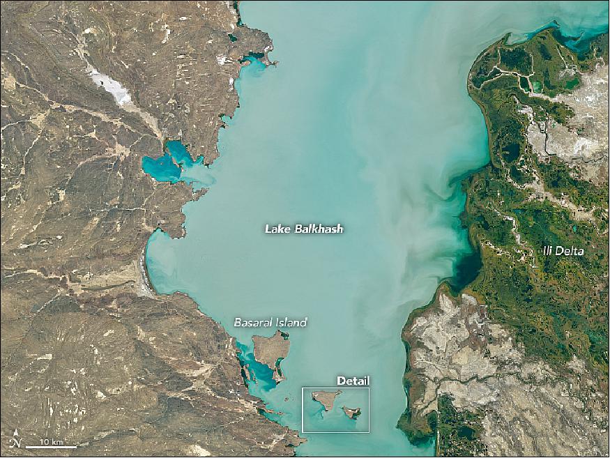
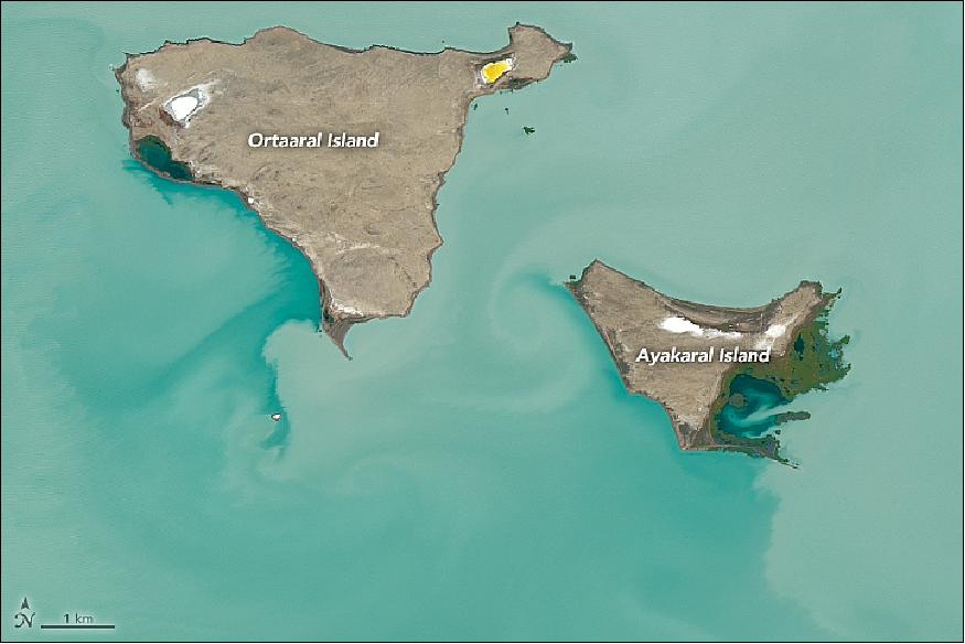
- If you were to cruise in a boat in the main part of the lake, you could count 43 islands with a total area of 66 km2, according to Zhanna Tilekova of Kazakh National Technical University, who has published research on the region's geoecology. However, those numbers can change. Tilekova noted that as water levels decline, new islands form and the area of existing islands grows. In the western part of the lake, Tasaral (north of this image) and Basaral islands are the largest. Ortaaral and Ayakaral islands are also relatively large (Figure 15). Vegetation, likely small brown shrubs (Saxaul), can grow on these islands. The white areas are likely salt pans.
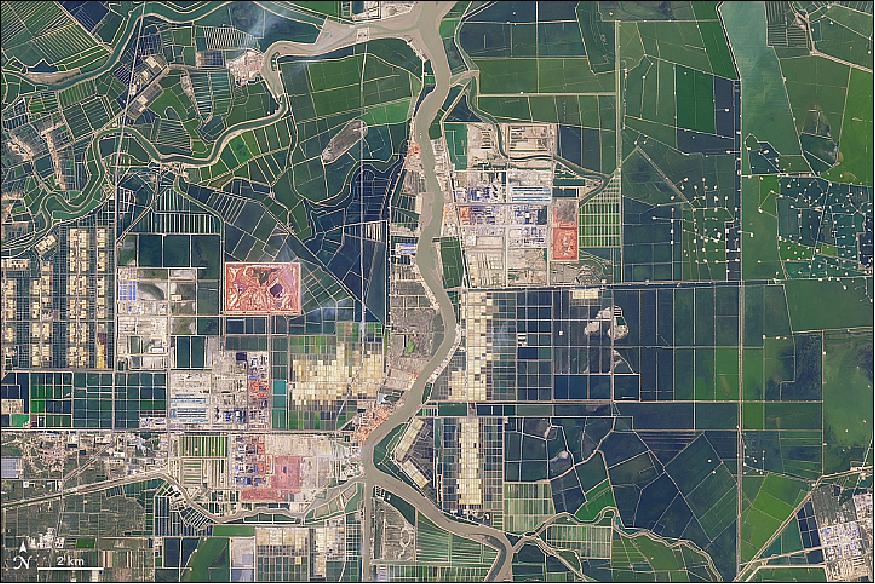
• October 29, 2017: In 1985, this part of Shandong Peninsula in eastern China was an open expanse of tidal mudflats frequented mainly by birds and other wildlife. By 2017, the landscape had been transformed into one that is intensely sculpted by human activity. 14)
- OLI (Operational Land Imager) on Landsat-8 captured this natural-color image on September 8, 2017 (Figure 17). The area falls within Binzhou, a prefecture in northern Shandong Province. Seen from above, the landscape is checkered with squares and rectangles, likely aquaculture ponds and brine pools used to produce salt. Dozens of drill pads for oil pumps are visible on the right side of the image. This area falls within the Shengli oil field, the second largest oil field in China.
- Heavy industry—likely oil-refining facilities—are visible near the center of the image. Landsat imagery shows that construction of these industrial facilities began in 2012. The drill pads were mostly established in the mid-1990s. Other major industrial products produced in Binzhou include garments, a fuel called coke, heavy machinery, and cement.
- In research that uses decades of Landsat imagery to determine where surface water has undergone the most change, this area stands out. Browse the Aqua Monitor and Surface Water Explorer to see how the distribution of surface water has changed in this part of China since the 1980s.
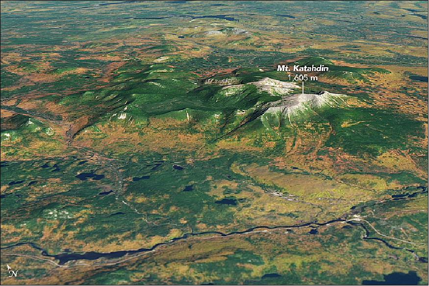
• October 22, 2017: As autumn progresses, so does the trail of color across New England. The reds, yellows, and oranges of the season typically emerge first on the deciduous trees and shrubs at higher latitudes and elevations. That was the case on October 13, 2017, when the Operational Land Imager (OLI) on Landsat-8 captured this natural-color image of foliage in north-central Maine. 15)
- The image of Figure 18 shows the mountainous part of Baxter State Park, an 200,000-acre (809 km2) area of protected wilderness. The summit of Mount Katahdin rises to 1,605 m, the tallest point in the state. Vegetation growth is stunted on the mountain's upper slopes and tablelands, which appear light tan. Moving down from the tree line you start to see evergreens, and then deciduous species with magnificent, colorful foliage. When the image was acquired, leaf color was at its local peak for 2017.
- "Typically, northern Maine reaches peak conditions the last week of September into the first week of October," according to the Maine Foliage Report. "The rest of the state's progression of color will start occurring from north to south in mid-October. Coastal Maine typically reaches peak conditions mid-to-late October."
- Leaf color appears around the same time every year, when daylight grows shorter and triggers plants to slow and stop the production of chlorophyll. But for the best color, leaves need dry weather and cooler temperatures. According to news reports, New England's foliage this year may not be as vibrant as other years. As of early October, many areas had not yet seen temperatures cool off much, causing leaves to go from green to brown.
- The Appalachian National Scenic Trail, generally known as the Appalachian Trail or simply the A.T., is a marked hiking trail in the Eastern United States extending between Springer Mountain in Georgia (Southern terminus) and Mount Katahdin in Maine (Northern Terminus). The trail is about 3500 km in length, claimed to be the longest longest hiking-only trail in the world. More than 2 million people are said to do at least a one day-hike on the popular trail each year. "Thru-hikers" attempt to hike the trail in its entirety in a single season — more than 2,700 people thru-hiked the trail in 2014. 16)
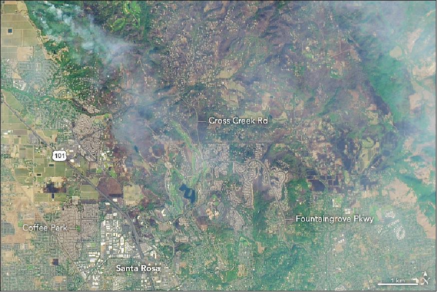
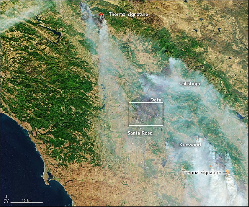
• October 13, 2017: Devastating wildfires have burned through California's wine country since October 8, 2017, taking dozens of lives and leaving thousands of people homeless. Even communities distant from the fires have been plagued by poor air quality, as the smoke plumes have darkened skies and canceled school and other activities across the region. 17)
- On October 11, OLI on Landsat-8 acquired the data for these false-color images of the fires near Santa Rosa and other communities in Northern California. The images are composites combining shortwave infrared, near-infrared, and green (OLI bands 6-5-3) with natural color (bands 4-3-2) and a thermal infrared signature (TIRS, band 10). These combinations make it easier to see through the smoke to the burn scars and the still-active fires.
- In the past week, 21 wildfires have ignited in Napa, Sonoma, Solano, and Mendocino counties and other communities north and east of San Francisco Bay. Fanned by northeasterly Diablo winds, the fires have collectively consumed at least 170,000 acres (265 square miles) of land—an area about half the size of the city of Los Angeles.
- The most prominent events include the Tubbs fire (between Santa Rosa and Calistoga, Figure 20), which has burned more than 34,000 acres; the Atlas fire (near Lake Berryessa, off the lower right of our image), which torched 44,000 acres; and the Redwood/Potter fires (near Mendocino National Forest, north of this scene) with 32,000 acres burned. Part of the Adobe fire (about 8,000 acres) appears in the lower right of the image, near Kenwood.
- CalFire and local officials reported that at least 3,500 homes and businesses have been destroyed, and thousands more are being threatened. Tens of thousands of people have evacuated, and thousands of firefighters have been sent to stop the spreading flames. As of the morning of October 12, most of the fires had little or no containment, according to CalFire bulletins, and "red flag warnings" were still being raised for fire weather with low humidity and high winds.
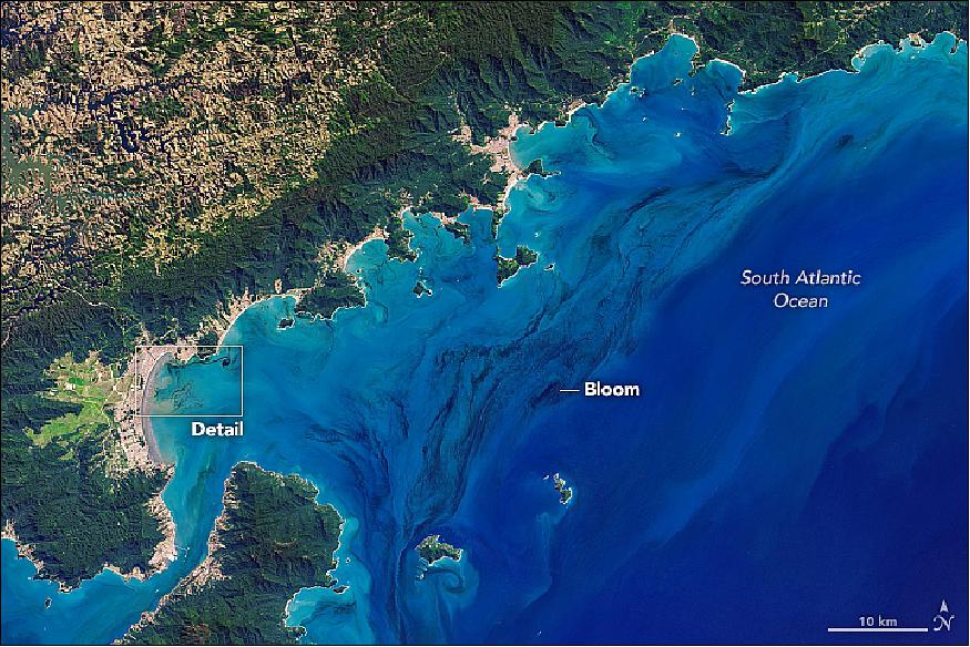
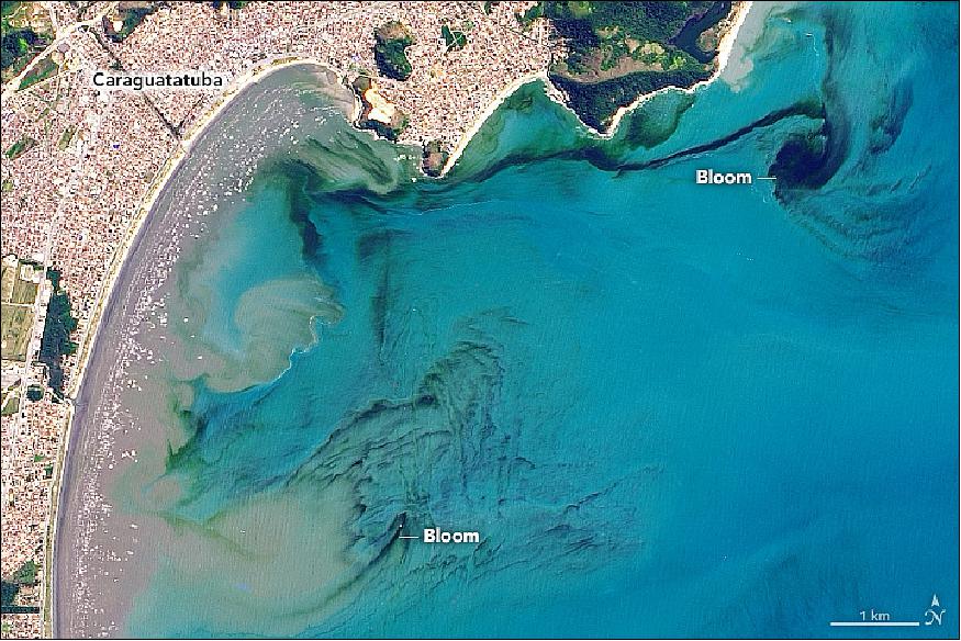
• September 10, 2017: In early September 2017, ocean scientists noticed something swirling in the waters off the coast of the Brazilian state of São Paulo. The sinuous threads of darkness amid the blue Atlantic Ocean were not caused by oil; they were the result of a phytoplankton bloom. 18)
- OLI on Landsat-8 captured the image of Figure 21 on September 5, 2017. Figure 21 is a wide view showing blooms spanning more than 100 km off of São Paulo state. The image of Figure 22 shows details of the bloom near Caraguatatuba. The dark colors are probably high concentrations of dinoflagellates, according to researchers at the University of São Paulo. Analyzing water samples collected from Caraguatatuba Bay and from the channel between the Ilhabela archipelago and the mainland, they identified the species as likely to be Gymnodinium aureolum.
- "But, this is a complicated species to identify," said Aurea Maria Ciotti, a scientist at the university's Center for Marine Biology. She and others are awaiting the results of additional tests to confirm the identification. "Blooms here are very uncommon—this is the first time for this species as far as we know."
- In January 2014, a bloom of a different species—Myrionecta rubra—appeared as dark patches that spanned about 800 km of the waters near Rio de Janeiro. Both the 2014 and 2017 blooms appear dark in satellite images for the same reason; the high concentration of heavily pigmented cells darken the water and less light is reflected directly back toward the satellite.
• September 8, 2017: The HLS (Harmonized Landsat Sentinel-2) project has released a new and improved version of its data sets. Landsat-8 and Sentinel-2 satellites have spectral and spatial similarities that make using their data together possible. When the data are used together observations can be more timely and accurate. Note: Sensor co-calibration efforts were underway prior to Sentinel-2A's launch. 19)
- Sentinel-2 and Landsat products represent the most widely accessible medium-to-high spatial resolution multispectral satellite data. Following the recent launch of the first out of two Sentinel-2 satellites, the potential for synergistic use of the two sources creates unprecedented opportunities for timely and accurate observation of Earth status and dynamics. Thus, harmonization of the distributed data products is of paramount importance for the scientific community. Activities to harmonize data products are on their way, yet more coordination is needed to allow the majority of users to easily and effectively include both data types into their work.
- The HLS project is an effort to "harmonize" the data of the two satellite programs so that they can be more easily used in unison. The ultimate goal is to obtain seamless 2-3 day global surface reflectance coverage at 30 meters that removes residual differences between the sensors due to spectral bandpass and view geometry. Currently the v1.3 HLS data set encompasses 82 global test sites that cover about 7% of the global land area.
- Using the processing power of the NASA Earth Exchange (NEX) computer cluster at NASA Ames, the HLS workflow atmospherically corrects data from the satellites, geographically tiles the Landsat data in a manor matching the Sentinel-2 tiling, and then corrects for different sensor view angles BRDF (Bidirectional Reflectance Distribution Function) and does a slight band pass adjustment for the Sentinel-2 data to create the harmonized 30 meter product.
- The new HLS version 1.3 expanded the number of geographic test sites, fixed a bug that was causing incorrectly calibrated coefficients to be used when calculating spectral reflectance and another bug in the BRDF calculation. Version 1.3 also changed the band combination of its quick-look browse images to follow the USGS standard format (SWIR-1, NIR, Red) and it added quality assessments on a per-site basis in addition to the previous per-tile availability.
- Currently, HLS data are only available for dates through April 30, 2017 because the HLS process relies on pre-collection L1T data.
- The next version of HLS will include a wall-to-wall harmonized product for North America, and will migrate to routine weekly processing. The project anticipates releasing the new version (v1.4) by early 2018.
- The HLS team includes researchers from NASA Goddard Space Flight Center, the University of Maryland, and NASA Ames Research Center.
• September 5, 2017: On January 17, 2017, a fire lit by a farmer in a swampy area along the Peruaçu River burned out of control and moved into the Peruaçu Environmental Preservation Area, a national park in the state of Minas Gerais, Brazil. From there, it proceeded to burn amidst grass, bushes, and palm trees (Mauritia flexuosa) for the past eight months. 20)
- Rather than producing big, orange flames and billowing plumes of smoke, this fire smoldered underground in dried out, carbon-rich soil and likely peat. In this part of the world, swampy soils near rivers are often drained to make them more suitable for growing crops. On August 11, 2017, OLI (Operational Land Imager) on Landsat-8 captured this image of the charred landscape (gray) that the fire left behind.
- "The fire spread slowly through soil and roots without any visible flames, but it was able to move up the hollow trunks of the Mauritia flexuosa and jump to the palm tree canopy," explained Jose Eugenio Cortes Figueira, a biologist at the Federal University of Minas Gerais who has been monitoring the fire.
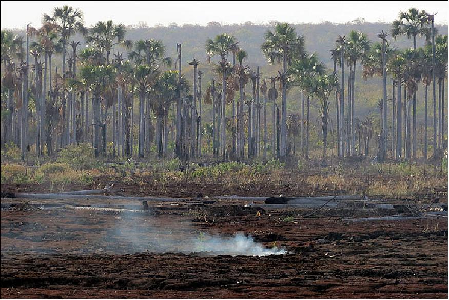
- In mid-August 2017, the burn scar was still smoldering and hundreds of palm trees had toppled over. The photograph of Figure 25, taken by Figueira, shows smoke seeping from the ground with several downed palm trunks behind it. As of mid-August, the fire had burned roughly 600 hectares of palm swamp along the river—in roughly the same area that had burned during a similar fire in 2014.
![Figure 24: The OLI image, acquired on Aug. 11, 2017, shows the burn scar left by a palm swamp fire in Brazil along the Peruaçu River. Rather than producing big, orange flames and billowing plumes of smoke, this fire smoldered underground in dried out, carbon-rich soil and likely peat. The fire spread slowly through soil and roots, but it was able to move up the hollow trunks of palm trees in the area and burn off the canopy [image credit: NASA Earth Observatory, image by Joshua Stevens, using Landsat data from the USGS, Story by Adam Voiland, with information from Jose Eugenio Cortes Figueira (Federal University of Minas Gerais) and Geraldo Wilson Fernandes (Federal University of Minas Gerais)].](/api/cms/documents/163813/4588098/LS82017-2013_Auto67.jpeg)
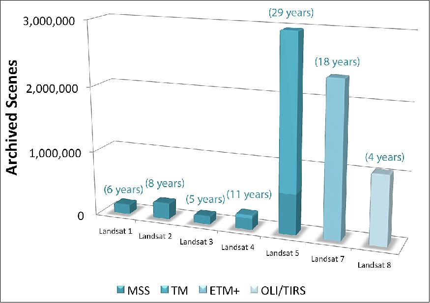
• September 1, 2017: Landsat-8, after collecting data for 4.5 years, has already added over a million images to the archive—this represents 14.8 percent of the entire 45-year Landsat data collection—and each day Landsat-8 adds another ~700 new scenes. 21)
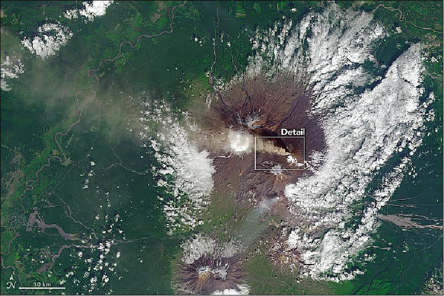
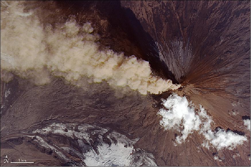
• August 24, 2017: The Kamchatka Peninsula's location along the Pacific Ring of Fire puts the peninsula in one of the most geologically restless areas on the planet. There are more than 100 active volcanoes on the peninsula, one of the highest concentrations of active volcanoes anywhere. 22)
- The most restless of these is Klyuchevskoy (also spelled Kliuchevskoi), a stratovolcano that rises 4,835 meters (15,862 feet) above sea level. According to geological and historical records, Klyuchevskoy has rarely been quiet since it formed about 6,000 years ago. Smithsonian's Global Volcanism Program details a steady stream of activity at Klyuchevskoy punctuated by eruptions every few years that often span months.
- True to form, satellites observed ash and volcanic gases puffing from Klyuchevskoy throughout much of August 2017. The Operational Land Imager (OLI) on Landsat 8 captured this image of a volcanic plume streaming west from the volcano on August 19, 2017. The plume is brown; clouds are white. Note in the broader view that there is also a smaller plume streaming from Bezymianny, a volcano to the south of Klyuchevskoy.
- Fewer than 300 people live within 30 km of Klyuchevskoy, so eruptions do not pose much risk to people on the ground. However, they can represent a hazard to aircraft if ash clouds rise to heights between 8 and 15 km. The ash plume was at a height of roughly 6 km on the day this image was collected, according to the KVERT (Kamchatka Volcanic Eruption Response Team).
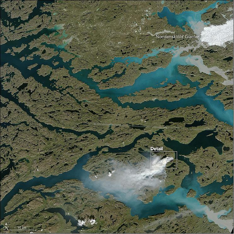
• August 12, 2017: Greenland is best known for its ice, but some remote sensing scientists found themselves closely tracking a sizable wildfire burning along the island's coast in August 2017. The fire burned in western Greenland, about 150 km northeast of Sisimiut. 23)
- Satellites first detected evidence of the fire on July 31, 2017. MODIS (Moderate Resolution Imaging Spectroradiometer) and VIIRS (Visible Infrared Imaging Radiometer Suite) on Suomi NPP collected daily images of smoke streaming from the fire over the next week. OLI (Operational Land Imager) on Landsat-8 captured these more detailed images (Figures 29 and 30) of the fire on August 3, 2017.
- While it is not unprecedented for satellites to observe fire activity in Greenland, a preliminary analysis by Stef Lhermitte of Delft University of Technology in the Netherlands suggests that MODIS has detected far more fire activity in Greenland in 2017 than it did during any other year since the sensor began collecting data in 2000.
- Fires detected in Greenland by MODIS are usually small, most likely campfires lit by hunters or backpackers. But Landsat did capture imagery of another sizable fire in August 2015. According to Ruth Mottram of the Danish Meteorological Institute (DMI), neither DMI nor other scientific groups maintain detailed records of fire activity in Greenland, but many meteorologists at the institute have heard anecdotal reports of fires.
- The blaze appears to be burning through peat, noted Miami University scientist Jessica McCarty. That would mean the fire likely produced a sharp increase in wildfire-caused carbon dioxide emissions in Greenland for 2017, noted atmospheric scientist Mark Parrington of the European Commission's Copernicus program.
- It is not clear what triggered this fire, though a lack of documented lightning prior to its ignition suggests the fire was probably triggered by human activity. The area is regularly used by reindeer hunters, and is not too far from a town with a population of 5,500 people.
- The summer has been quite dry. Sisimiut saw almost no rain in June and half of the usual amount in July. That may have parched dwarf willows, shrubs, grasses, mosses, and other vegetation that commonly live in Greenland's coastal areas and made them more likely to burn.
- Fires emit a soot-like material called black carbon. It is likely that winds will transport some of this material east to the ice sheet where it will contribute to a line of darkened snow and ice along the western edge of Greenland's ice sheet. This area is of interest to climate scientists because darkened snow and ice tends to melt more rapidly than when it is clean.
• July 2017: The Landsat-8 OLI instrument continues to be remarkably stable over its four years on orbit. Significant change is only apparent in the Coastal Aerosol band (band 1) and this approximately 1% change in response is currently being corrected in operational data processing. 24)
- In addition, all the on-board calibration devices are working well, and with the exception of a few small (<1%) degradations in the devices used most frequently, have not degraded. The availability of the multiple devices allows identifying the degrading devices and deciphering instrument change from calibrator change.
• On July 23, 2017, the Landsat Program celebrateed forty-five years of continuous Earth observation. NASA — working in cooperation with the U.S. Department of the Interior (DOI) and its science agency, the USGS — launched the first Landsat satellite (originally named Earth Resources Technology Satellite 1) on July 23, 1972. 25)
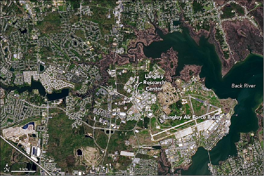
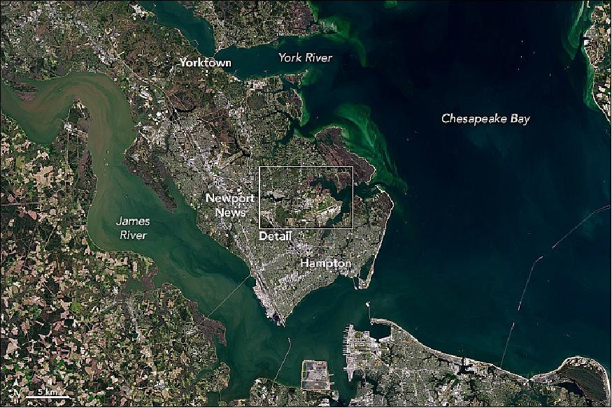
• July 18, 2017: Something happened 100 years ago that changed forever the way we fly. And then the way we explore space. And then how we study our planet. That something was the establishment of what is now known as NASA Langley Research Center (LRC), which is commemorating its 100th anniversary in 2017. 26)
- Just three months after the United States entered into World War I, Langley Memorial Aeronautical Laboratory was carved out of coastal farmland near Hampton, Virginia, as the nation's first civilian facility focused on aeronautical research. The goal was, simply, to "solve the fundamental problems of flight." Under the direction of the National Advisory Committee for Aeronautics (NACA), ground was broken for the center on July 17, 1917.
- From the beginning, Langley engineers devised technologies for safer, higher, farther, and faster air travel. More than 40 state-of-the-art wind tunnels and supporting infrastructure have been built over the years, and researchers use those facilities to develop many of the wing shapes still used today in airplane design. Better propellers, engine cowlings, all-metal airplanes, new kinds of rotorcraft and helicopters, faster-than-sound flight—these were among Langley's many groundbreaking aeronautical advances.
- During World War II, Langley tested planes like the P-51 Mustang in the nation's first wind tunnel built for full-sized aircraft. Langley later partnered with the military on the Bell X-1, an experimental aircraft that would fly faster than the speed of sound. Follow-on research would extend the reach of American aeronautics into supersonics and hypersonics. By 1958, NACA would become NASA, and Langley's accomplishments would soar from air into space.
- Over the past half century, LRC has contributed significantly to the development of rockets and to the spacecraft testing and astronaut training of the Mercury, Gemini, and Apollo programs. In particular, astronauts practiced Moon landings here with the lunar lander. Langley also led the unmanned Lunar Orbiter initiative, which not only mapped the Moon, but helped choose the spot for the first human landing. With the Viking 1 landing in 1976, Langley led the first successful U.S. mission to the surface of Mars. All along, the center and its researchers have contributed to the study of Earth via satellite and through instruments flown on the space shuttles, space station, and NASA aircraft.
- Over the past half century, LRC has contributed significantly to the development of rockets and to the spacecraft testing and astronaut training of the Mercury, Gemini, and Apollo programs. In particular, astronauts practiced Moon landings here with the lunar lander. Langley also led the unmanned Lunar Orbiter initiative, which not only mapped the Moon, but helped choose the spot for the first human landing. With the Viking 1 landing in 1976, Langley led the first successful U.S. mission to the surface of Mars. All along, the center and its researchers have contributed to the study of Earth via satellite and through instruments flown on the space shuttles, space station, and NASA aircraft.
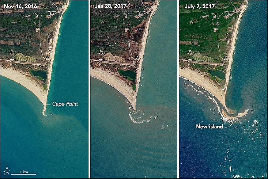
• July 12, 2017: The waters off of North Carolina's barrier islands have been called a "graveyard of the Atlantic." Countless ships have wrecked here, due to the area's treacherous weather and currents and its expansive shoals. These shoals are, by definition, usually submerged. But occasionally parts of them can rise above sea level. 27)
- These natural-color images, acquired by OLI (Operational Land Imager) on the Landsat-8 satellite, show the shoal area off of Cape Point at Cape Hatteras National Seashore—the site of a newly exposed shoal nicknamed "Shelly Island." The first image was captured in November 2016. When the second image was acquired in January 2017, waves were clearly breaking on the shallow region off the cape's tip. The site of those breakers is where the island eventually formed, visible in the third image captured in July 2017. The new island measures about a mile long, according to news reports.
- "What exactly causes a shallow region to become exposed is a deep question, and one that is difficult to speculate on without exact observations," said Andrew Ashton, a geomorphologist at the Woods Hole Oceanographic Institution. "A likely process would be a high tide or storm-driven water elevation that piled up sediment to near the surface, and then water levels went down exposing the shoal. Waves then continue to build the feature while also moving it about."
- While the exact mechanism for the formation of Shelly Island this year is mostly unknown, the phenomenon is not uncommon. Cape Lookout, the next cape down the barrier islands (to the southwest, beyond this image) has had several islands form on its shoal over the past decade or two.
- The shoreline and cape tips along North Carolina's barrier islands are constantly in motion. Cape tips are sculpted by waves and currents that hit from all directions. Meanwhile, sediment is carried up and down the coastline and often deposited near the cape tips. Each cape has a so-called "cape-associated shoal" lurking underwater. These submerged mounds of sand can extend for tens of kilometers. They are also very shallow, rising to anywhere from 10 meters to a few meters below the surface in places.
- "Tidal flows moving up and down the coast are diverted by the capes and result in a net offshore current at cape tips and deposition at the shoals," Ashton said. "Occasionally, a portion of the shoal becomes exposed and forms an island."
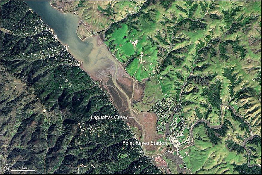
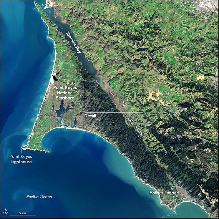
• June 17, 2017: There is an obvious difference between the dark green coniferous forests that dominate the western shore of Tomales Bay and the lighter green grasslands on the east side (Figure 35). But the differences between the two shores run much deeper than the vegetation. - Tomales Bay lies about 50 km northwest of San Francisco, along the edges of two tectonic plates that are grinding past each other. The boundary between them is the San Andreas Fault, the famous rift that partitions California for hundreds of miles. 28)
- To the west of the Bay is the Pacific plate; to the east is the North American plate. The rock on the western shore of the Bay is granite, an igneous rock that formed underground when molten material slowly cooled over time. On the opposite shore, the land is a mix of several types of marine sedimentary rocks. In Assembling California, John McPhee calls that side "a boneyard of exotica," a mixture of rock of "such widespread provenance that it is quite literally a collection from the entire Pacific basin, or even half of the surface of the planet."
- As the plates shift, the ground west of the San Andreas Fault moves northward. On average, movement along the fault averages about 3 to 5 cm per year—about the speed that fingernails grow. However, that movement is anything but steady. The two plates tend to lock together until extreme amounts of pressure build up. When the pressure reaches a breaking point, an earthquake sends the plates lurching. During the Great 1906 San Francisco Earthquake, a road at the head of Tomales Bay was offset by nearly 6 meters.
- In Figure 36, you can see that the direction of the fault follows the orientation of Tomales Bay, running from the head of the Bay through Olema Valley toward Bolinas Lagoon.
• June 7, 2017: Forests, grasslands, deserts, and mountains are all part of the Patagonian landscape that spans more than a million km 2 of South America. Toward the western side, expanses of dense, compacted ice stretch for hundreds of kilometers of the Andes mountain range in Chile and Argentina. Glaciologist Eric Rignot described these icefields as "one of the most beautiful places on the planet." Their beauty is also apparent from space. 29)
- The two lobes of the Patagonian icefields—north and south—are what's left of a much more expansive ice sheet that reached its maximum size about 18,000 years ago. The modern icefields are just a fraction of their previous size, though they remain the southern hemisphere's largest expanse of ice outside of Antarctica.
- "The rapid thinning of the icefield's glaciers illustrates the global impact of climate warming," said Rignot, of NASA's Jet Propulsion Laboratory and the University of California-Irvine. "We have shown that Patagonia glaciers experience some of the world's most dramatic thinning per unit area, more than Alaska or Iceland or Svalbard or Greenland."
- The northern remnant is the smaller of the two icefields, covering about 4,000 km2 (about a quarter the size of the southern icefield). On April 16, 2017, the Operational Land Imager (OLI) on Landsat 8 captured this rare cloud-free image of the entire North Patagonian Icefield (Figure 37).
- While the northern icefield is smaller than its southern counterpart, it still has 30 significant glaciers along its perimeter. Ice creeps downslope through mountain valleys and exits the through so-called "outlet glaciers." Many come to an abrupt end on land, while others terminate in water. The water-terminating glaciers San Rafael and San Quintín are the icefield's largest.
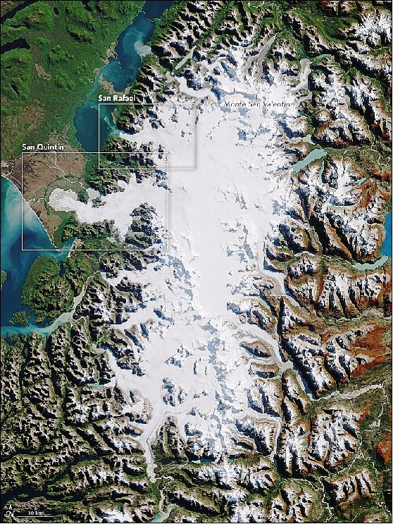
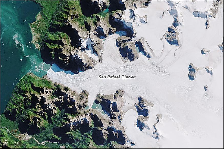
- The San Rafael Glacier starts near the western flank of Monte San Valentin—the tallest summit in Patagonia—and drains westward into Laguna San Rafael. The lagoon is ringed by a ridge of debris, called a moraine, shoveled into place by the glacier in the past when it was much larger. Visitors to the area in the late 1800s described the glacier as having a large bulbous front, called a piedmont lobe, that spread out well into the lagoon. Since then, the glacier has receded and is no longer lobe-like, though it still actively sheds icebergs from its front in a process known as calving. San Rafael is one of the most actively calving glaciers in the world.
- Part of the reason why this glacier sheds so many bergs is because of its speed. "Flowing" at a speed of 7.6 km/year, San Rafael is the fastest-moving glacier in Patagonia and among the fastest in the world.
- It is also the icefield's only glacier to come into contact with ocean water. Seawater from the Pacific enters the lagoon through the Golfo Elefantes, which connects to the lagoon via the Rio Tempanos (Iceberg River). At 46.7 degrees south latitude, San Rafael is the closest glacier to the equator in the world to connect to the sea.
- There was a point when seawater did not reach the glacier. "It used to be a lagoon with fresh water," said Rignot. "Then an earthquake in the 1960s lowered the ground and connected the lagoon with the ocean waters (the passage for seawater is only a few meters deep)."
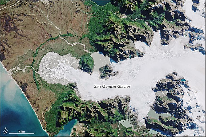
- San Rafael's "twin" is the San Quintín glacier immediately to the southwest. This glacier currently ends in a piedmont lobe, and illustrates what San Rafael looked like before it receded. Until 1991, the glacier terminated on land, but with the glacier's retreat, the basin has filled in with water to form a proglacial lake. (Note that the lake water is barely distinguishable from the ice due to its milky color).
- San Quintín does not flow as fast (1.1 km/ year) or calve as many bergs as San Rafael, but it is an impressive glacier on its own, standing as the second-largest in the North Patagonian Icefield. Together with San Rafael, the glaciers drain 37 percent of the icefield.
- Like its twin, San Quintín has been receding dramatically. Researchers have shown that between 1870 and 2011, the glacier lost 14.6 percent of its area. For comparison, San Rafael lost 11.5 percent during the same period.
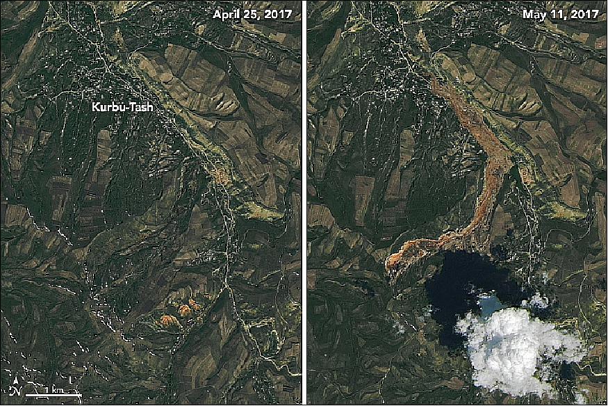
• May 30, 2017: In April 2017, a hillside saturated by melting snow and rainfall collapsed near the village of Kurbu-Tash in southern Kyrgyzstan. Over the following weeks, a slow-moving river of fine-grained soil flowed down a valley and engulfed dozens of homes. 30)
- On May 11, 2017, the OLI (Operational Land Imager) on the Landsat-8 satellite captured an image (right) of the landslide deposit. Freshly exposed soil is tan. For comparison, the image on the left shows the same area on April 25, 2017. The landslide transported 2.8 million m3 of soil, according to Kyrgyzstan's Ministry of Emergency Situations.
- People living in the foothills of the Tien Shan mountains in southern Kyrgyzstan face an unusually high risk of landslides. Several factors contribute to the elevated risk, including the presence of active faults, steep terrain, and the presence of landslide-prone soil types. Loess, for instance, is involved in many landslides in this region because the fine-grained soil becomes quite unstable when saturated with water. Heavy bouts of rain, the melting of snow, and small earthquakes often trigger slides. The risk is particularly high in the spring, when heavy rainfall is most likely. Since the area is densely populated, landslides take lives and destroy many homes each year.
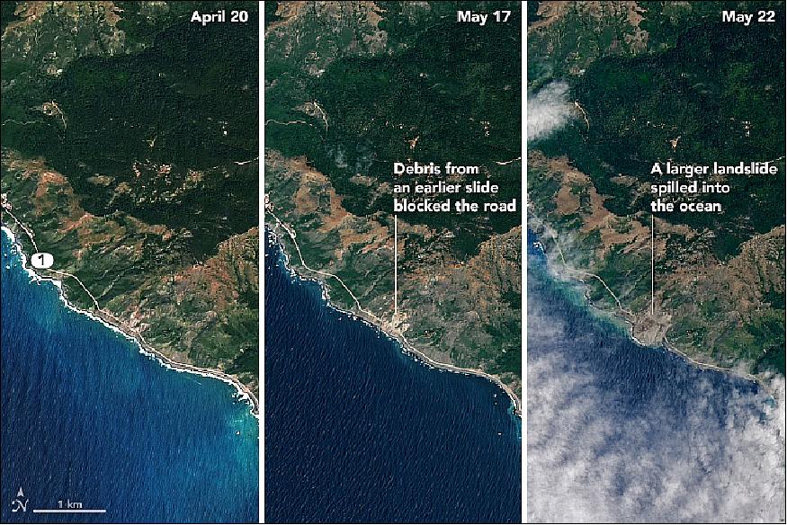
• May 25, 2017: A large landslide has strewn debris over a stretch of California's Highway 1. On the night of May 20, 2017, more than a million tons of rocks and dirt spilled over the roadway, according to the California Department of Transportation. 31)
- OLI ( Operational Land Imager) on Landsat 8, acquired images of the area on April 20 and May 22, 2017. The center image, acquired by a the MSI (Multispectral Imager) on the European Space Agency's Sentinel-2 satellite, shows the same location as it appeared after a previous, smaller landslide this spring.
- "This is a large slide preceded by smaller slides, which is not uncommon," said Thomas Stanley, a geologist and researcher for NASA, in an email. "Much of the California coastline is prone to collapse, so it's fortunate that this landslide happened in an unpopulated location." In 2015, the Monterey County Environmental Resource Policy Department rated parts of the nearby coast as highly susceptible to landslides.
- The latest landslide covered roughly one-third of a mile of the scenic route in 10 to 12 meters of rubble. The highway will remain closed for the foreseeable future, according to Caltrans.
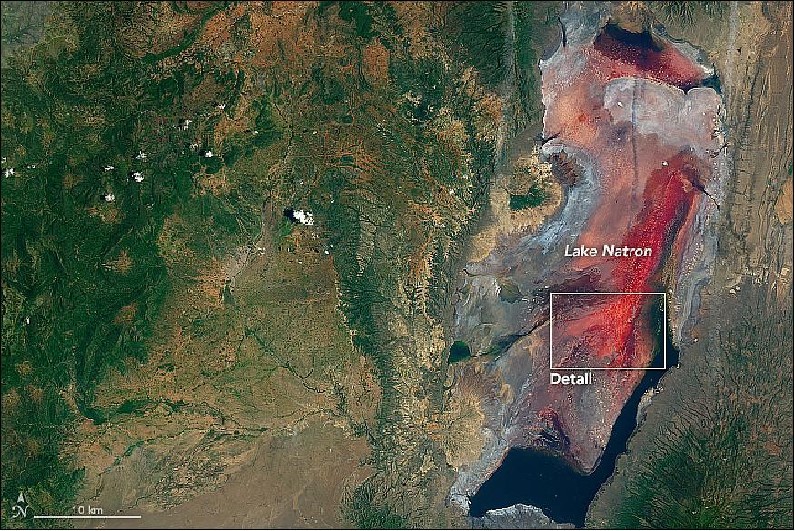
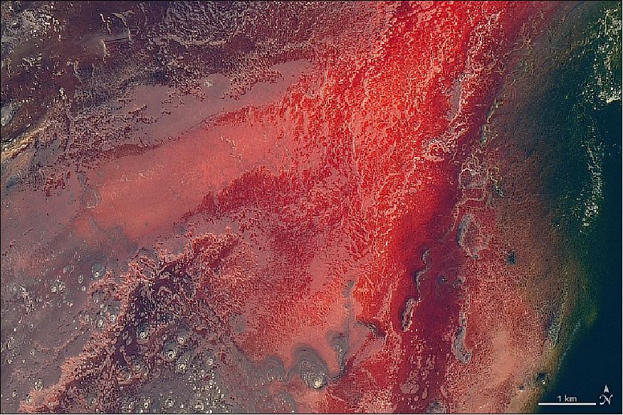
• May 8, 2017: Not many people venture near the shores of Lake Natron in northern Tanzania. The lake is mostly inhospitable to life, except for a few species adapted to its warm, salty, and alkaline water. 32)
- But you don't need to visit the lake in person to see its stunning, seasonal color. OLI (Operational Land Imager) on Landsat 8 captured these natural-color images of Lake Natron and its surroundings. They show the lake on March 6, 2017, very early in the rainy season that runs from March to May. In these images, you can see the deepest water along the perimeter of the lake bed, the location of lower-elevation lagoons.
- The lake is a maximum of 57 km long and 22 km wide. The climate here is arid. High levels of evaporation have left behind natron (sodium carbonate decahydrate) and trona (sodium sesquicarbonate dihydrate). The alkalinity of the lake can reach a pH level of greater than 12. In a non-El Niño year, the lake receives less than 500 mm of rain. Evaporation usually exceeds that amount, so the lake relies on other sources—such as the Ewaso Ng'iro River at the north end—to maintain a supply of water through the dry season.
- But it's the region's volcanism that leads to the lake's unusual chemistry. Volcanoes, such as Ol Doinyo Lengai (about 20 km to the south), produce molten mixtures of sodium carbonate and calcium carbonate salts. The mixture moves through the ground via a system of faults and wells up in more than 20 hot springs that ultimately empty into the lake.
- While the environment is too harsh for most common types of life, there are some species that take advantage of it. Small, salty pools of water can fill with blooms of haloarchaea—salt-loving microorganisms that impart the pink and red colors to the shallow water. And when the waters recede during the dry season, flamingos favor the area as a nesting site, as it is mostly protected from predators by the perennial moat-like channels and pools of water.
- Lake Natron is a salt and soda lake in the Arusha Region of northern Tanzania. The lake is close to the Kenyan border and is in the Gregory Rift, which is the eastern branch of the East African Rift. The lake is within the Lake Natron Basin, a RAMSAR Site wetland of international significance.
- The lake is the only regular breeding area in East Africa for the 2.5 million lesser flamingoes, whose status of "near threatened" results from their dependence on this one location. When salinity increases, so do cyanobacteria, and the lake can also support more nests. These flamingoes, the single large flock in East Africa, gather along nearby saline lakes to feed on Spirulina (a blue-green algae with red pigments). Lake Natron is a safe breeding location because its caustic environment is a barrier against predators trying to reach their nests on seasonally forming evaporative islands. Greater flamingoes also breed on the mud flats.
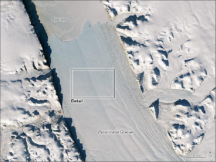
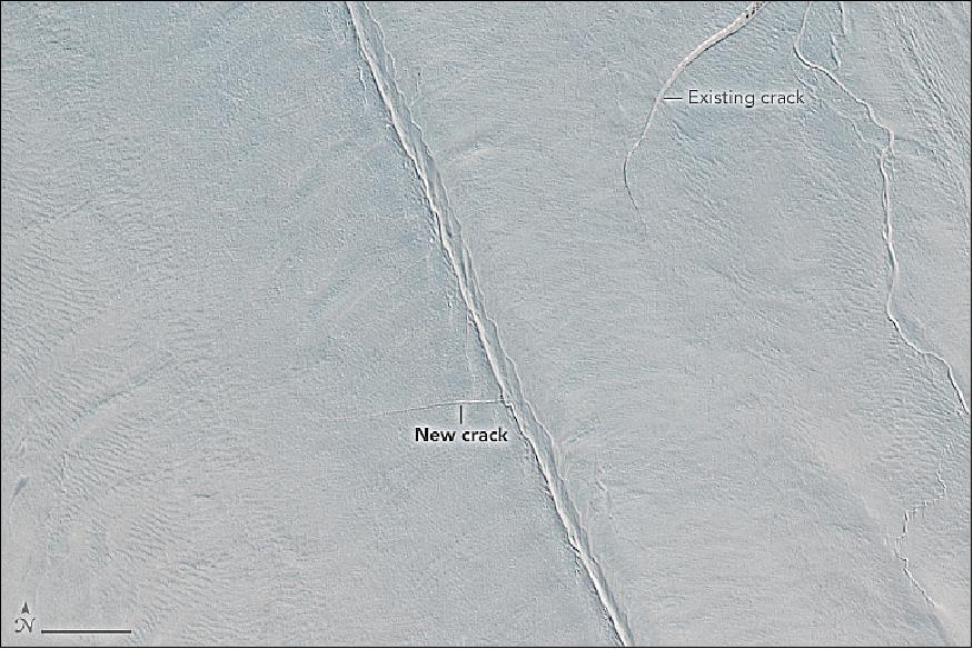
• April 19, 2017: The ice atop Greenland is not static. It slowly flows toward the coast and enters the ocean via outlet glaciers that ring the giant island. Petermann Glacier is one such "river" of ice. Like most glaciers that come in contact with the sea, Petermann has been known to periodically shed, or calve, icebergs. A new crack on the glacier has glaciologists watching Greenland's northwest coast closely. 33)
- The new crack, or "rift," is visible in these images acquired on April 15, 2017, with OLI (Operational Land Imager) on Landsat 8. The image of Figure 44 shows a wide view of the glacier, including its front—where the glacier's floating tongue meets the fjord's ice-covered sea water. The image of Figure 45 shows a detailed view of the rift.
- "Rifting and calving are normal," said Kelly Brunt, a glaciologist at NASA/GSFC ( Goddard Space Flight Center). "However, if this new rift crosses Petermann and calves a good chunk of ice, it would be the third such relatively large iceberg from this system in about seven years." It remains to be seen whether that will happen. Brunt points out that the rift currently appears to end at a feature running down the center of the glacier. "That's pretty typical," she said, citing similar occurrences on ice shelves in Antarctica.
- This new rift could eventually work its way through the feature in the center of the glacier. Or, the new rift could be met by an old rift—visible in the upper-right part of the detailed image—as it works its way from the northeast side of the glacier fjord. "But there is really no telling at this point," Brunt said.
- The day before the satellite images were acquired, Brunt flew with NASA's Operation IceBridge, an airborne science mission that conducts important surveys of snow and ice near Earth's poles. The flight had a number of goals, including an overflight of the recently discovered rift.
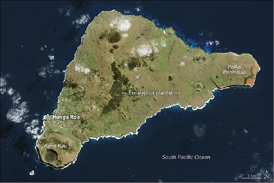
• April 16, 2017: This remote volcanic island has intrigued generations of scholars. Famed for its monolithic statues, Easter Island is shrouded in mystery. Its population, once sizable, collapsed (Figure 46). 34)
- "The clearest example of a society that destroyed itself by overexploiting its own resources," is how University of California Los Angeles geographer Jared Diamond once described it. But the island's history may not be as clear-cut as Diamond suggests. While scientists agree that broad-scale deforestation occurred here at some point, the verdict is still out on what exactly caused the downfall of the Rapanui people.
- Scholars do agree on one thing: the island once looked very different than it does today. Called Rapa Nui by its original inhabitants, it takes its English name from the day Europeans arrived: April 5, 1722—Easter Sunday. Dutch navigator Jacob Roggeveen reported a few thousand people living there at the time. He described this island, more than 3,000 km west of South America, as "exceedingly fruitful, producing bananas, potatoes, sugar-cane of remarkable thickness."
- Unbeknownst to Roggeveen, the indigenous population he encountered was just a fraction of its former size. Scholars estimate that between 15,000 to 20,000 people lived on Rapa Nui at the peak of its habitation. A thick cover of palm trees once shaded its hills, which are now fringed by low-lying vegetation.
- The extinct Terevaka volcano dominates the landscape, which also includes Poike and Rano Kau volcanoes and a number of smaller volcanic features such as lava tubes. Tufts of clouds pepper the sky overhead and a thick white outline along the island's southern edge indicates strong waves crashing against its shores. The Poike Peninsula, which juts out to the east, appears orange in places, a result of erosion exposing the brightly colored volcanic soil. The largest stand of trees, a eucalyptus plantation, was planted by people. Authorities hope reforestation efforts will help protect the island against the scouring wind.
- About 5,000 people live on Easter Island today, and thousands of tourists come to see the anthropomorphic "moai" statues each year. Amid strain from a rising population, the island faces challenges ahead. It has no sewer system and continues to draw on a limited freshwater supply.
• March 31, 2017: This month, 20 Landsat scenes were ingested by the USGS Hazard Data Distribution System to provide data for Charter activations: 35)
The International Charter is a system that supplies free satellite imagery to emergency responders anywhere in the world. The Charter concept is this: a single phone number is made available to authorized parties providing 24/7 contact to a person who can activate the charter. Once activated, a project manager takes charge. The project manager knows what satellite resources are available, how to task them to collect data, and how to quickly analyze the collected data to create impact maps for first responders. These maps, provided to responders for free, often show where the damage is and where crisis victims are, allowing responders to plan and execute relief support.
You can think of the Charter as a one-stop-shop for impact maps—an essential resource, since in many cases satellite data are the only practical method to assess current ground conditions after a disaster.
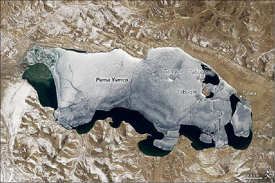
• March 18, 2017: Several hundred lakes dot the expansive Tibetan Plateau. With the average plateau elevation exceeding 4,500 meters above sea level, its lakes are among the highest in the world.
- Puma Yumco in Lhozhag County is one of the larger lakes in southern Tibet. A small village along the eastern edge of the lake—Tuiwa—is reportedly one of the highest administered settlements in the world, sitting at an elevation of 5,070 meters. Tuiwa's economy centers on raising livestock (sheep and yaks), tourism, and textiles. Though there are fish in the lake, they are considered sacred and are not eaten by most Tibetans. - Lake Puma Yumco is 32 km long and 14 km wide and covers an area of 880 km2.
- Every winter, villagers herd thousands of sheep across the lake's frozen surface to two small islands, where the soil is more fertile and the forage is better in the winter.
- While the rhythms of life have remained largely unchanged in Tuiwa for many decades, researchers have used satellites to track subtle changes at Puma Yumco and other lakes throughout the plateau. One team has found that the number of lakes on the Tibetan Plateau has increased by 48 percent, and the surface area of the water has increased by 27 percent between the 1990s and 2015. For Puma Yumco, the size of the lake dropped a bit between the 1970s and 1990s, but has risen since then, primarily because of an increase in precipitation.
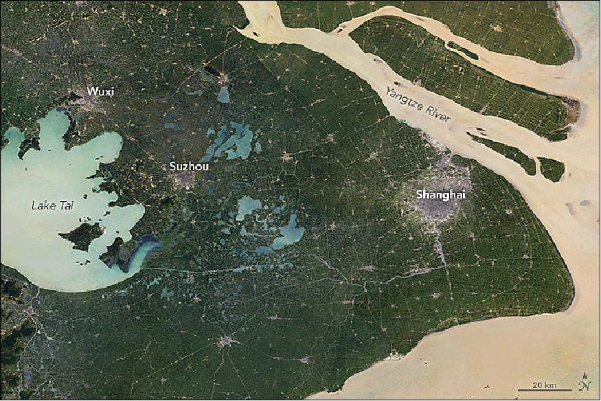
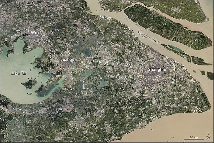
• March 17, 2017: Geographers who have studied the growth of China's cities over the past four decades tend to sum up the pace of change with one word: unprecedented. In 1960, about 110 million Chinese people—or 16% of the population—lived in cities. By 2015, that number had swollen to 760 million and 56%. -For comparison, the entire population of the United States was about 325 million people as of March 2017. 36)
- The surge in urbanization began in the 1980s when the Chinese government began opening the country to foreign trade and investment. As markets developed in "special economic zones," villages morphed into booming cities and cities grew into sprawling megalopolises. Perhaps no city epitomizes the trend better than Shanghai. What had been a relatively compact industrial city of 12 million people in 1982, had swollen to 24 million in 2016, making it one of the largest metropolitan areas in the world.
- For more than four decades, Landsat satellites have collected images of Shanghai. The composite images of Figures 48 and 49 show how cities in the Yangtze River Delta have expanded since 1984. Note how Suzhou and Wuxi have merged with Shanghai to create one continuous megalopolis (Figure 49).
- These "best-pixel mosaics" are made up of small parts of many images captured over five-year periods. The first image is a mosaic of scenes captured between 1984 and 1988; the second shows the best pixels captured between 2013 and 2017. This technique makes it possible to strip away clouds and haze, which are common in Shanghai.
- A 2015 World Bank report noted that 7,734 km2 in the Yangtze River Delta Economic Zone—which includes Shanghai, Suzhou, Wuxi, and several other cities—became urban between 2000 and 2010. That is an area equivalent to 88 Manhattans. During that period, population in that zone increased by 21 million people.
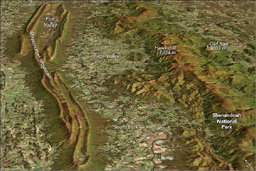
• March 15, 2017: Along the western border of Virginia, two roughly parallel ridges—one of which is the backbone of Shenandoah National Park and the other part of George Washington National Forest—rise above the rolling lowlands of the Shenandoah Valley. Despite being just a few kilometers apart, the ridges show some marked differences (Figure 50). 37)
- With a perimeter of smooth, straight crests encircling a valley, Massanutten Mountain has the look of a flat-bottomed canoe. Shenandoah National Park's portion of the Blue Ridge, in contrast, has a more textured, irregular, and knobby shape; it looks more like a spine, with a dendritic network of gullies descending from its main crest.
- The two ridges look different due to distinct geological histories. The rock underneath Shenandoah National Park is largely igneous, meaning it was created when magma or lava cooled and solidified. Some of the oldest rocks in the park are granites that formed deep underground about 1.1 billion years ago when continents collided and pushed up a mountain range during the Grenville orogeny. Major outcrops of granite are located east of Shenandoah's highest crest and dominate peaks such as Old Rag and Mary's Rock.
- About 500 million years later, the tectonic tides had shifted. Instead of continents colliding, they were pulling apart. As the crust thinned and rifts formed, volcanoes sprang up and spilled lava across the land surface. This laid down layer upon layer of basalt, a type of igneous rock that cools quickly and thus has small mineral crystals. When exposed later to the high temperatures and pressures associated with the collision of tectonic plates, the basalt metamorphosized into metabasalt. This greenish rock, known in this area as the Catoctin Formation, makes up much of the Blue Ridge's highest crest, including peaks like Hawksbill, Stony Man, Mount Marshall, and Hightop.
- As the rift widened, it eventually connected with the ocean and was filled by a narrow, shallow sea. At its bottom, sedimentary rocks began to form as layers of sand, mud, and material from sea life began to rain down on the sea floor and become sandstone, shale, and carbonate rock.
- The landscape we see today was set up by one more cycle of continents slamming into each other—a collision between North America and Africa about 300 million years ago known as the Alleghanian orogeny. While building mountains that were once as tall as the Himalayas, the Alleghanian orogeny thrust the older igneous rocks (once the root of the Grenville range) upward and squeezed them into a curved bulge called an anticline, putting older rock layers quite close to the surface. The same collision squeezed and folded the nearby rocks of the Shenandoah Valley and Massanutten into a concave depression called a syncline that kept the youngest sedimentary rocks quite close to the surface.
- With the rock layers in place, erosion played the final role in sculpting the modern landscape. Rivers such as the Shenandoah's South Fork wore away relatively soft and weak types of sedimentary rock (the shale and carbonates) to create low-relief areas such as the Shenandoah Valley, Page Valley, and Fort Valley. Erosion-resistant, quartz-rich sandstone remained to give Massanutten Mountain its distinctive shape. To the east, the erosion-resistant igneous-based rocks of the Blue Ridge tower over Shenandoah Valley, Massanutten Mountain, and the rest of the Piedmont.
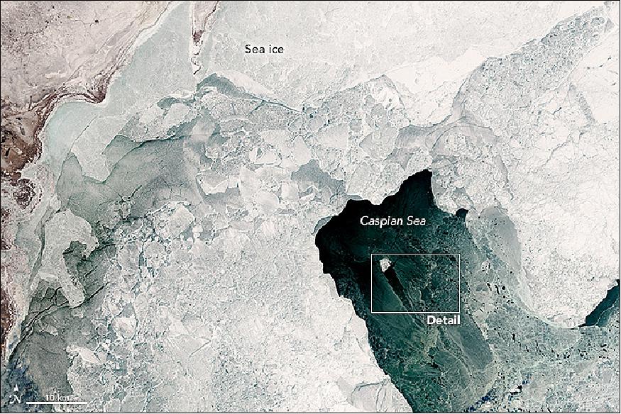
• March 1, 2017: The Caspian Sea stretches about 1,000 km from Kazakhstan to Iran. In the north, temperatures are colder, and the water is fresher (less saline) and shallower. As a result, northern areas are more prone to freezing in wintertime. 38)
- The image of Figure 51 shows the northwestern Caspian where it meets western Kazakhstan. The brown areas are part of the Volga Delta. Just offshore, in the shallowest parts (only meters deep), a well-developed expanse of consolidated ice appears white. Farther offshore, a large field of old, hummocked, white and gray-white ice has detached. (When pieces of ice are pushed together, some ice is forced upward and downward into so-called ‘hummocks.') This ice is slowly drifting in a giant polynya which is covered by young, thin ice (nilas).
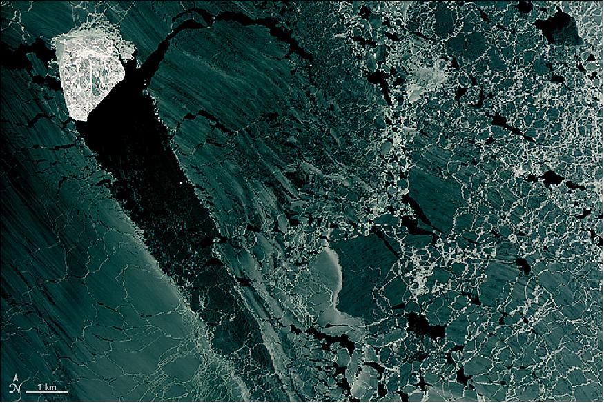
- The image of Figure 52 shows a detailed view of the nilas ice, which appears dark. Perhaps most notable, however, is the white, diamond-shaped piece of ice parked right in the middle. "This ‘island' of white ice is most probably a piece that detached from the ice field," said Alexei Kouraev, a scientist at the Laboratory of Geophysical and Oceanographic Studies (France). He notes that a likely point of origin is the "dent" of similar size in the boundary of the white ice (mid-right in the image of Figure 51).
- It might look like that ice diamond is on the move, cutting a path through the thinner cover. But it's more likely that the chunk of ice broke away from the thicker sea ice and became grounded—anchored to the bottom of the sea. The grounded ice (‘stamukha' in Russian) is not moving, according to Kouraev. Instead, the wind is pushing the thin ice around this grounded ice, creating a ‘shadow' of open water behind it.
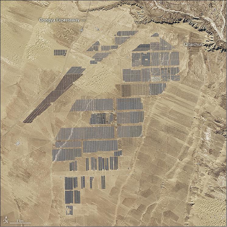
• February 16, 2017: In the past few years, the title of "largest solar farm in the world" has been a rather short-lived distinction. For a period in 2014, the Topaz Solar Farm in California topped the list with its 550 MW facility. In 2015, another operation in California, Solar Star, edged its capacity up to 579 MW. By 2016, India's Kamuthi Solar Power Project in Tamil Nadu was on top with 648 MW of capacity. — As of February 2017, Longyangxia Dam Solar Park in China was the new leader, with 850 MW of capacity. 39)
- By January 5, 2017, solar panels covered 27 km2 of the Qinghai province in China (Figure 53). According to news reports, there were nearly 4 million solar panels at the site in 2017. The rapid expansion at Longyangxia coincides with China's fast-growing solar power sector. In 2016, China's total installed capacity doubled to 77 GW. That pushed the country well ahead of other leading producers—Germany, Japan, and the United States—to become the world's largest producer of solar power. However, those three countries (and several others) produce more solar power per person.
- It is unlikely that Longyangxia will remain the largest solar park in the world for long. A project planned for the Ningxia region in China's northwest will have a capacity of 2,000 MW when it is finished, Bloomberg reported.
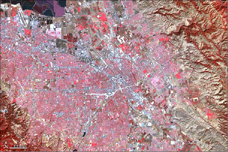
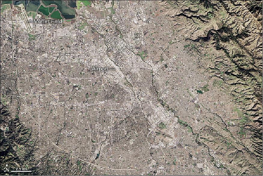
• February 5, 2017: Image comparison of Silicon Valley observed by Landsat-1 in 1972 and by Landsat-8 in 2016.
By the middle of the 20th Century, Silicon Valley was already "on the map." This part of California's Santa Clara Valley drew its nickname from the raw material being used in the region's growing semiconductor industry. The area at the south end of San Francisco Bay became a magnet for scientists and for technology companies, so by the time the new Landsat-1 satellite caught a glimpse in 1972, urban sprawl had already replaced many of the valley's orchards. 40)
- While the two images of Figures 54and 55 don't show much change in the development of the landscape, they clearly show the development of the technology behind Landsat's satellite sensors. The false-color image of Figure 54 was acquired on October 6, 1972, with the MSS (Multispectral Scanner System) on Landsat-1; the natural-color image of Figure55 was acquired on November 18, 2016, by the OLI (Operational Land Imager) on Landsat-8.
- The most obvious improvement is the spatial resolution. Over the past 45 years, you have certainly noticed similar improvements in your electronics and imaging products. Better spatial resolution is the reason you can now see blades of grass in a televised football game and the fine lines on your face in a smartphone photo. In short, there is a lot more detail visible in the 2016 image than in the 1972 image. Both are displayed at a resolution of 45 m per pixel. The MSS image is relatively blurry, however, because the sensor's spatial resolution was just 68 x 83 m. The OLI image appears crisper because the instrument can resolve, or "see," objects down to about 30 m (15 m in some cases).
- The 2016 image also has better radiometric resolution, which means the newer instrument is more sensitive to differences in brightness and color. OLI uses 4,096 data values to describe a pixel on a scale from dark to bright. MSS used just 64. More data ultimately translates to the features in the image appearing smoother.
- Finally, the images are very different colors because the wavelengths (color) of light used to compose the images are from different parts of the spectrum. Both images were composed using red and green wavelengths. The image of Figure 54, however, uses near-infrared. False-color images like this one (MSS bands 6, 5, 4) are still produced with modern instruments because they are useful for distinguishing features such as vegetation, which appears red in the top image.
- In contrast, the OLI image does not show near-infrared (although the instrument does have the capability). Instead, it includes blue, a color that MSS was not designed to sense. This combination (OLI bands 4, 3, 2) produces a natural-color image similar to what your eyes would see.
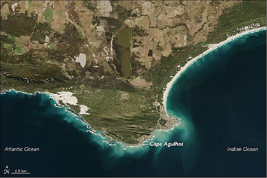
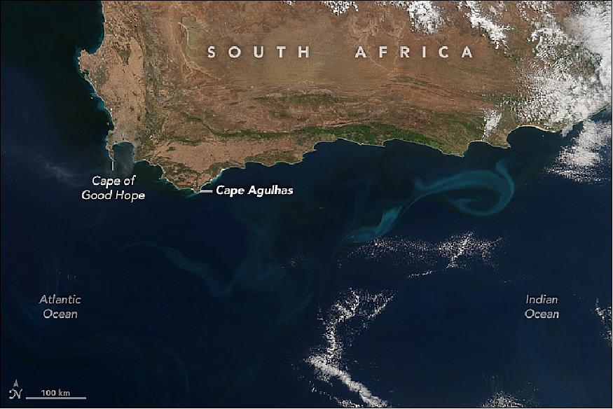
• January 27, 2017: Mariners have long considered the waters off Africa's southern tip to be treacherous. After decades of failed attempts to navigate around the continent, Portuguese explorers took to calling one of its southerly promontories the Cape of Storms (it was later renamed the Cape of Good Hope). Cape Agulhas , Africa's southernmost point, is Portuguese for Cape of Needles. Historians think the name may be a reference to the needle-like rock formations and reefs along its coast. 41)
- The convergence of two ocean currents—one warm and one cold—in the shallow waters of Agulhas Bank produces turbulent and unpredictable waters. Warm water arrives from the east on the fast-moving Agulhas Current, which flows along the east coast of Africa. Meanwhile, the cooler, slower Benguela Current flows north along Africa's southwestern coast. That means navigating around the tip of South Africa requires mariners to sail against ocean currents on both sides of the continent.
- Eventually, they learned to stay well out to sea as they rounded the Cape of Good Hope and Cape Agulhas, but not before failed attempts had littered the area's reefs with wrecked ships. Even in modern times, shipwrecks are relatively common in the turbulent water of Agulhas Bank, where colliding currents regularly spin off rogue waves, eddies, and meanders.
- The instability and churning does have one benefit. As water masses stir the ocean, they draw nutrients up from the deep, fertilizing surface waters to create blooms of microscopic, plant-like organisms (phytoplankton) in the open ocean. The phytoplankton feed a robust chain of marine life that makes Agulhas Bank one of the richest fishing grounds in southern Africa.
• January 4, 2017: Around Lake Thurmond, a large reservoir that straddles Georgia and South Carolina, something is not right with the birds. The lake is full of vegetation — particularly an invasive aquatic plant known as Hydrilla verticillata — and the area is full of birds that are distressed or dying. 42)
- Scientists have deduced that the birds are consuming a toxic cyanobacteria that lives on Hydrilla verticillata. The toxin causes a neurodegenerative disease and ultimately death in the water birds that ingest it. Eagles don't eat the plants, but they do prey on other birds. And many eagles have been found dead in the vicinity of Lake Thurmond.
- Hydrilla is tenacious. It grows in fresh water on every continent except Antarctica, and it has been found in at least 30 states in the U.S. The plant tolerates a wide range of temperature, nutrient, salinity, and turbidity conditions, and it can grow as fast as one inch per day. In Lake Thurmond, the plant can be found in 11,200 of the lake's 71,000 acres. The U.S. Army Corps of Engineers has used herbicides to temporarily control the plant's growth at boat ramps and swimming areas, but the impact on birds has encouraged investigation into treatments that would be more widespread and long-term.
- To help lake managers know where to focus management efforts, researchers at the University of Georgia developed a new way to assess the distribution of Hydrilla across the lake. The project was part of NASA's DEVELOP program, in which recent college graduates and early career professionals use NASA satellite observations to address an environmental or public policy issue. On October 18, 2015, the Operation Land Imager on the Landsat-8 satellite acquired an image (Figure 58) of Lake Thurmond. Blue overlays on the Landsat image show the extent of Hydrilla that month. The map is based on a model developed by the team, derived from Landsat-8 imagery and ground-based measurements.
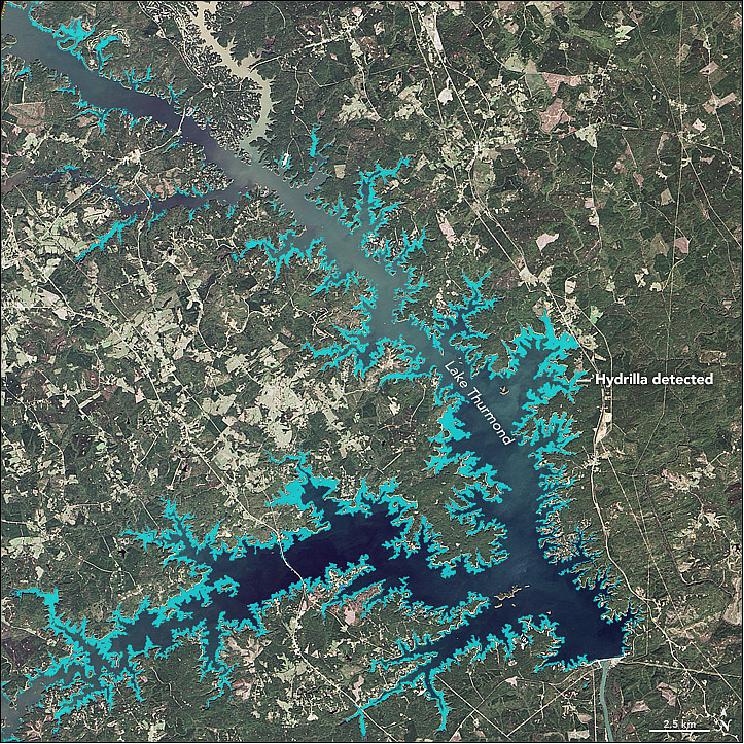
- Hydrilla grows best under specific water and light conditions. The model accounts for those parameters, represented in this series of four images (Figure 59). The most important factor is the water's transparency (top left). By lowering a Secchi disk into the water and measuring the depth at which it is no longer visible, scientists can estimate the water's transparency. In this map, the darkest orange areas are transparent and yellow areas are turbid (murky). Highly transparent regions are more suitable for Hydrilla.
Note: a Secchi desk, created by Angelo Secchi in 1965, is a plain white, circular disk 30 cm in diameter used to measure water transparency in bodies of water. The disc is mounted on a pole or line, and lowered slowly down into the water. The depth at which the disk is no longer visible is taken as a measure of the transparency of the water. This measure is known as the Secchi depth and is related to water turbidity.
- From the transparency measurement, the team derived other parameters, including the gradual loss of light at depth, or "light attenuation" (top-right), the percentage of light penetrating the column of water (bottom-left), and the maximum depth at which Hydrilla colonize (bottom-right). The new model integrates all of these parameters to determine the ideal locations for Hydrilla growth. According to the DEVELOP team, the model will "act as the foundation for later models intending to predict future locations in need of Hydrilla management."
• December 21, 2016: At first glance, a river's course may seem fixed and unchanging. In truth, the path is a perpetual work-in-progress that, in some cases, can shift dramatically in a short span of time. This is especially true in the Moxos plains of northern Bolivia. In this tropical area east of the Andes, several rivers meander through a swampy landscape of savanna, forests, and ponds. While studying three decades of satellite imagery of this area, geographer Umberto Lombardo of the University Pompeu Fabra in Barcelona, Spain, noticed a particularly striking example of rapid change on a stretch of the Maniqui River. 43)
- OLI (Operational Land Imager) on Landsat-8 captured four false-color images between 2013 and 2016 (Figure 60). These images were assembled using red, green, and shortwave infrared light. The use of infrared light makes it easier to distinguish between silt-laden water and bare land. Water absorbs infrared light, while plants and bare earth reflect it. As a result, areas with standing water appear blue, while bare land appears light brown. Forests are bright green; savanna is pink-brown.
- "Images like this underscore how much and how quickly small- and medium-size rivers in this part of the world change," said Umberto Lombardo. Earlier research on larger rivers in the Amazon had suggested that big shifts in a river's path usually coincide with major flooding associated with La Niña, a cyclical cooling of ocean temperatures in the equatorial Pacific. But after systematically combing through three decades of satellite imagery and the paths of 12 small and medium-sized rivers in the southern Amazon, Umberto found no obvious connection to La Niña. Instead, he found that the course of small rivers tended to be in a regular state of change regardless of La Niña cycles.
- Umberto's findings have on-the-ground implications. Authorities should be prepared for the possibility that indigenous communities living along small rivers may have to be resettled if rivers shift in the coming years. Also, a planned road linking Villa Tunari to San Ignacio de Moxos may be destroyed or regularly flooded without careful planning, he explained.
• December 2016: The in-orbit performance of Landsat-8 continues to be outstanding, currently acquiring around 740 scenes per day, and several Antarctic and Arctic off-nadir requests have recently been fulfilled with no impact on routine imaging. Operational and data processing solutions have been implemented to mitigate the impact of the anomaly in Landsat-8's TIRS (Thermal Infrared Sensor) SSM (Scene Select Mirror). All affected data have been reprocessed and nominal TIRS data collection and processing have been restored. 44)
- Landsat MSS (Multispectral Scanner) Improvement Plan: There are efforts to improve the Landsat MSS archive, including MSS reflectance-based calibration, adjustment of minimum and maximum radiance values to minimize saturation, updating of gain-trend models, and derivation of a bulk correction factor to minimize attitude bias. Overall, the processing and model updates being implemented will help increase the number—as well as the geometric and radiometric quality—of MSS Level-1T scenes. Currently, the plan is to begin collection-processing for MSS in the summer of 2017.
- Landsat-8 TIRS Reprocessing Status: Ron Morfitt reported of how image measurements from geometric calibration are being used to correct the SSM issue, which caused TIRS images to be shifted out of alignment with OLI by as much as 500 m. Overall, the new TIRS processing model is working well, with registration accuracy of around 20 m when telemetry and calibration data are available.
- Matt Montanaro and Aaron Gerace provided an update on the stray-light correction algorithm being developed for TIRS on Landsat-8. Montanaro explained how stray light entering the optical path from outside the direct field-of-view is causing significant nonuniform banding in the TIRS bands 10 and 11. The approach to correct this issue uses TIRS data to estimate the out-of-view signal, based on in-scene statistics. Initial validation results based on comparison with underpass data from the MODIS (Moderate Resolution Imaging Spectroradiometer) on Terra are encouraging. Although more testing is planned over land and low-temperature regions of Antarctica, the LST (Landsat Science Team) recommended moving toward operational implementation of the developed stray-light correction algorithm. The current plan is to implement the algorithm during Collection 1 reprocessing, which is slated to begin in the fall of 2016.
The NASA–USGS Landsat mission and European Space Agency's Sentinel-2 missions have collaborated to produce a Harmonized Surface Reflectance Product. The data products from these missions represent the most widely accessible medium-to-high spatial resolution multispectral satellite data in the world. Following the launch of the Sentinel-2A satellite on June 23, 2015, the potential for synergistic use of the two sources creates unprecedented opportunities for timely and accurate observation of Earth status and dynamics. Thus, harmonization of the distributed data products is of paramount importance for the scientific community. Activities to harmonize data products are on their way, yet more coordination is needed to allow the majority of users to easily and effectively include both data types into their work. |
• December 14, 2016: Earth's ice is changing, from mountain glaciers to ice sheets to ice shelves. For the most part, land-based ice has been shrinking, and the very definition of a "glacial pace" has changed within our lifetimes. Now researchers have the tools to see those changes every few weeks and at scales as small as 5 meters — the technique is known as feature tracking. 45) 46)
- Using freely available data from the Landsat 8 satellite, scientists are working to provide a near-real-time view of every large glacier and ice sheet on Earth. A group of scientists from the National Snow and Ice Data Center (NSIDC), the University of Alaska–Fairbanks, the University of Bristol, and the Jet Propulsion Laboratory (JPL) have started the GoLIVE (Global Land Ice Velocity Extraction) project , a NASA-funded effort to better understand how ice flow is changing worldwide.
- "We are now able to map how the skin of the ice is moving," said Ted Scambos, senior research scientist at NSIDC and lead for the GoLIVE project. "From now on, we're going to be able to track all of the different types of changes in glaciers. There's so much science to extract from the data." The effort was described at the 2016 fall meeting of the American Geophysical Union.
- Evidence strongly suggests that the loss of ice from glaciers and ice sheets has been the largest contributor to sea level rise over the past three decades, with waters rising at a global average rate of 3.3 mm/year. By examining changes in ice flow in combination with data on ocean and atmospheric changes, the researchers hope to determine what causes ice masses to change and how much ice will flow into the ocean. The satellite-based approach is particularly valuable in remote landscapes, where ground- and airplane-based observations are expensive, dangerous, and intermittent.
- In Alaska and Canada's Yukon Territory, for instance, most glaciers are so remote that speedup events can go unnoticed for months until a pilot flies over the region and reports disrupted ice, notes Mark Fahnestock of the University of Alaska. The map of Figure 61, based on an analysis by GoLIVE investigators, shows the velocity of ice in southeastern Alaska near Malaspina and Hubbard glaciers.
- "By measuring ice flow all the time, we can identify a surge as it starts, providing an entirely new way to follow this phenomenon," Fahnestock said. "We can also follow large seasonal swings in tidewater glaciers as they respond to their environment. Scientists need to see all of this variability in order to identify trends."
- Automation has been key to this ice velocity mapping effort. Landsat 8 collects images of roughly 700 sunlit parcels of the planet every day; over the course of 16 days, it observes the entire land surface of Earth in multiple visible and infrared wavelengths. This means scientists can view changes in the same spot on Earth every 16 days (or 32, 48, 64, etc., as cloud cover allows).
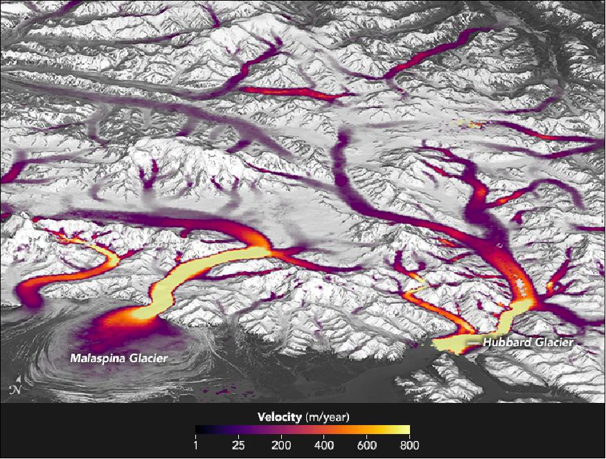
- It also means there is a huge amount of data to process and analyze. From 2013 to 2016, Landsat-8 collected thousands of images from Antarctica alone. The globes of Figure 62 show how many times Landsat-8 passed over a given icy parcel in 2015 alone. As many as 150 to 200 images were collected over the brightest yellow and green areas, while purple areas had just a handful of useful images because of frequent cloud cover and fewer orbital passes. Due to the nature of the satellite's polar orbit, areas in the far north and south can be imaged more frequently (when there is sunlight).
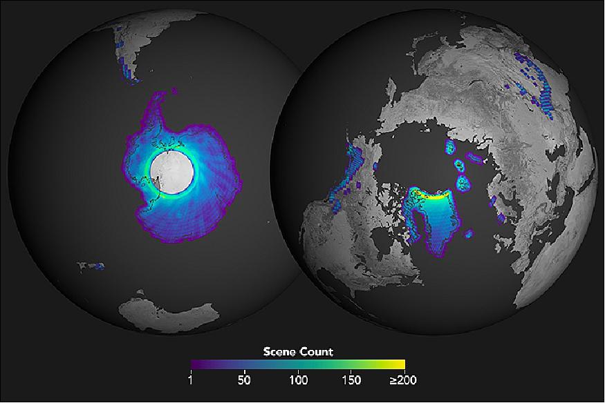
- The imaging system on Landsat-8 is far more sensitive than previous Landsat sensors, distinguishing far more subtle differences in shading and surface texture. The GoLIVE team has written software that allows researchers to follow these subtle features, like bumps or dune-like patterns on ice surfaces. By comparing images of the same location on different dates, researchers can track individual features and determine the speed of the surface flow. "The question is: how sensitive are these ice sheets to changes in the atmosphere and the ocean?" said Alex Gardner of JPL. "We could wait and see, or we could look to the past to help inform what is most likely to happen in the future."
- Gardner has been looking closely at Antarctica, with ice velocities represented in the map of Figure 63. He is working to combine the new Landsat 8 ice-flow data with prior maps of the continent's glacier flow in the hopes of understanding decadal changes across the entirety of the ice sheet. Almost 2,000 km3 of ice flows into the Southern Ocean from Antarctica each year.
- Twila Moon, an ice scientist at the University of Bristol, is using the global maps to expand her research in Greenland. With the new database, she can study the movements of more than 240 glaciers, nearly all of the outlets from the ice sheet. And with Landsat-8 making an overpass every 16 days, she has an opportunity to detect seasonal changes and cyclical patterns.
- While most glaciers speed up in the warmer summer months, Moon has found several that slow down dramatically in the mid- to late-summer. "We can group these glaciers by looking at the similarities in their behavior," Moon said. "It's providing an opportunity to get at the underlying drivers of why they change." With measurements of what the seasonal shifts do to glacier speed, scientists can extrapolate what might happen to those glaciers as global temperatures continue to climb.
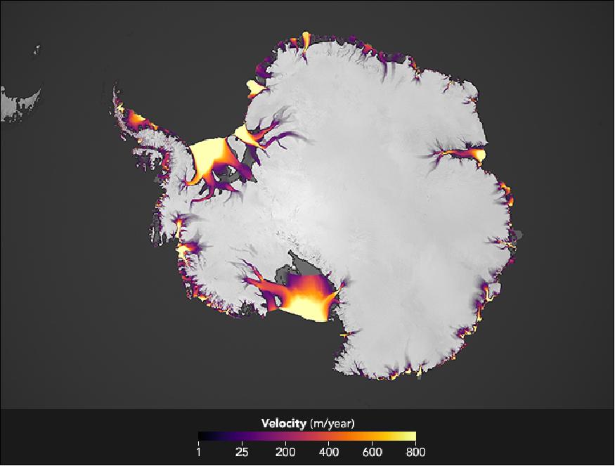
• November 19, 2016: In Landsat images of the Tafilalt oasis of southeastern Morocco, dozens of thin lines run across the desert from the Anti-Atlas mountains toward the town of El Jorf. These are qanats (khettaras in Moroccan)—ancient underground water channels designed to transport water down slopes without active pumping. 47)
- Most wells involve digging a vertical shaft downward until it reaches the water table, and then hauling or pumping the water up to the surface. Qanats consist of gently inclined horizontal tunnels dug into sloping terrain. When the horizontal tunnel hits the water table, gravity causes water to simply flow downhill in the channel toward outlets at the base of the slope.
- While the channels that convey the water lay below the surface, the access shafts used for construction and maintenance are visible above ground. The access shafts are often dug near or through large earthen mounds made of material excavated during construction of the vertical shafts and channels.
- From above, these earthen mounds form long chains that appear as relatively continuous lines at Landsat's 30 m/pixel spatial resolution.
• October 29, 2016: Kiruna, the largest underground iron ore mine in the world, has been in operation since 1900. But recent years have brought change for the residents of the nearby town. In the coming decade, the 23,000 people and their homes and businesses will move three kilometers away. 48)
- Resource extraction is crucial for the town's existence and economic wellbeing. But the steady development of mine shafts continues to weaken the ground there. In 2004, the mine's operator, the LKAB (Luossavaara-Kiirunavaara Company), announced that development of the mine has threatened the structural integrity of the town's buildings. Some of them, including Kiruna's historic red church, will be taken apart and reassembled at the new location.
- OLI (Operational Land Imager) on the Landsat-8 satellite captured this image (Figure 65) of the Kiruna mine, town, and nearby airport on October 10, 2016. The green vegetation is marbled with yellow, likely the result of birch forests and deciduous shrubs changing color. A dusting of snow whitens some hilltops in the image. The Sun's low angle on the southern horizon casts long shadows on the north sides of the hills.
- The Kiruna orebody is one of the world's largest magnetite-apatite deposits. Sweden, the biggest iron producer in Europe, owes its reserves to volcanic activity many thousands of years ago, according to a paper in Nature. 49)
• October 6, 2016: A special issue of the journal Remote Sensing of Environment details the improved capabilities and mission role of Landsat 8, the latest satellite in the world's longest, continuous program of Earth observation. 50) 51)
- Now available to the public, the compendium of 23 published papers describes how Landsat 8 is the most capable of the seven operational Landsat missions and highlights how Landsat 8's enhanced performance and new capabilities enable better science and research results. The selected articles cover topics from how the instrument's performance gives higher quality electromagnetic measurements to how its improved geometry allows for the tracking of moving ice sheets.
• October 14, 2016: Glaciers cover 11% of Iceland's landscape, the largest being the Vatnajökull – known as the Vatna Glacier in English – which at 8000 km2 is also the largest glacier in Europe (Figure 66). Up to 1 km thick, the Vatna ice cap has about 30 outlet glaciers – many of which are retreating owing to warming temperatures. 52)
- A number of volcanoes lie underneath this ice cap, including the infamous Grímsvötn, which caused disruption of northern European air traffic in recent years following eruptions and the spread of ash plumes. This volcano is visible as a black arc on the central-left side of the image. In 1996 an eruption of Grímsvötn caused some of the overlying glacial ice to melt. The water then broke out of the ice cap and flooded the nearby outwash plain, causing millions of dollars' worth of damage.
- In the upper-central part of the image, in an area known as the Holuhraun lava field, we can see a bright orange strip of lava through a crack in the surface. This type of elongated volcanic eruption is known as a fissure vent, and usually occurs without any explosive activity.
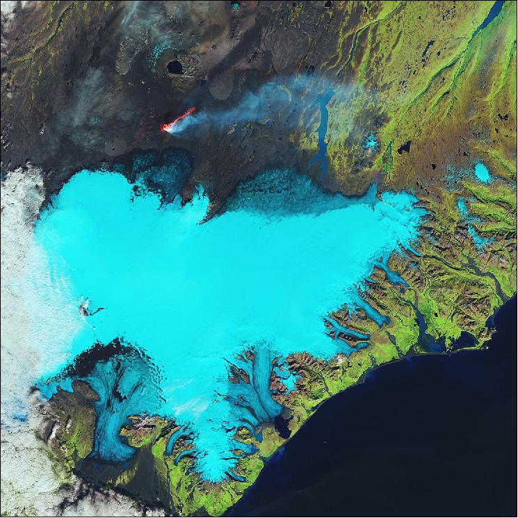
• September 21, 2016: Today the Landsat project celebrates the 50th anniversary of Secretary of the Interior Stewart Udall's 1966 announcement of "Project EROS (Earth Resources Observation Satellites)". Udall's vision paved the way for what we today know as Landsat, and gave the world the confidence to create satellite systems to monitor our planet with a new perspective. 53)
- Secretary Udall's vision to create "a program aimed at gathering facts about the natural resources of the Earth from earth-orbiting satellites" was an idealistic goal at the time, but on July 23, 1972, the first Earth Resources Technology Satellite (ERTS) was launched from Vandenberg Air Force Base in California. In 1975, it was renamed Landsat 1. Since then, six more Landsat satellites have followed, collectively capturing millions of images of Earth, and creating an impressive archive that has been available at no charge since 2008.
• September 21, 2016: In late July 2016, an illegal campfire gave rise to the Soberanes fire that grew near the California coast between Monterey and Big Sur. The wildfire continued burning in the Los Padres National Forest through August. As of late September, it was still not fully contained. The Landsat-6 satellite acquired the image of the area on September 15, 2016 (Figures 67 and 68, same image with different spectral bands). 54)
- When these images were acquired, the fire had burned 435 km2 and was 55 percent contained. Some of the smoke from the fire hung low in the local valleys, most notably on September 18 after a temperature inversion set in. An air quality report called the air "unhealthy" at sites near the fire including Carmel Valley, Cachagua, and Tassajara.
- Not all of the smoke, however, stayed local. The Ozone Mapper Profiler Suite (OMPS) on Suomi-NPP (Suomi National Polar-orbiting Partnership) satellite observed smoke fanning out to the southwest over the Pacific Ocean and inland to the east and northeast.
- By September 20, the fire was 71 percent contained and had burned 490 km2. New evacuations were in place after winds carried embers across the containment line and started a new "spot" fire measuring less than 1 km2.
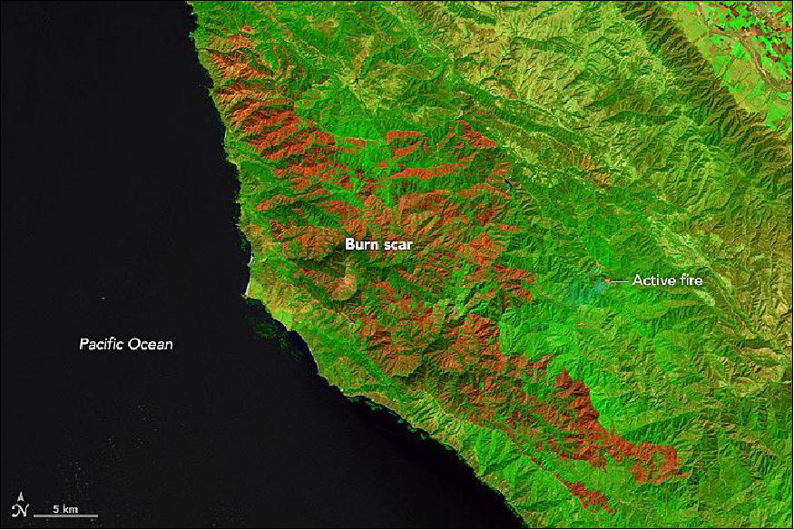
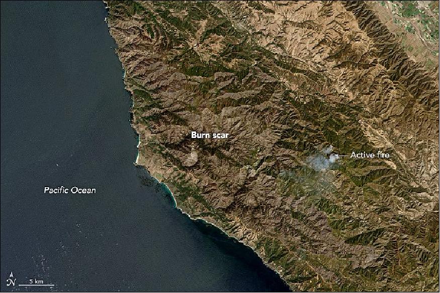
• August 25, 2016: This week marks the 100th anniversary of the National Park Service. We are celebrating this milestone with a gallery of images. On most summer days, a trip to North Carolina's Outer Banks means a peaceful day at the beach soaking up the sun and playing in the waves. But there is evidence all around that this beach is not always so serene. The very existence of these barrier islands is due to the power of wind and water. 55)
- Figures 69 and 70 show a segment of the barrier islands in the vicinity of Cape Hatteras National Seashore. The park's origins date back to the 1930s, when Congress authorized the creation of this first "national seashore park" in the United States. It wasn't until 1953 that the National Park Service acquired enough land to establish the park, and another five years before facilities were in place and the park could formally open.
- Stanley Riggs, a scientist who in the mid 1960s developed the coastal and marine science program at East Carolina University, pointed out some notable features. Skinny parts of the island chain, which appear mostly white without any green vegetation, are "simple" barrier islands. These areas are generally eroding and thinning. The shoreline continues to recede and weak spots form, at which point water from the Atlantic Ocean can break through and form an inlet.
- The year that these images were acquired was a relatively quiet one for storms. In other years, however, hurricanes and nor'easters have opened multiple inlets in a single season. Within a year or two after an inlet opens up, a flood tide delta typically forms behind it and continues the natural cycle of island rebuilding. That cycle is influenced, however, by the human development and maintenance of structures such as highway 12—the road that runs like a spine down the length of North Carolina's barrier islands.
- In contrast, the green vegetated areas along the islands are usually wider and older "complex" barrier islands. The second image shows a detailed view of one such area at Cape Hatteras. In this view, you can see parallel east-west ridges that have built up over time behind the tip of the cape. The relative height of the dunes and distance from the ocean have allowed forests to grow. These are also the more protected and therefore urbanized parts of the island chain.
- Still, the wind and waves take a toll, eroding the east-facing shoreline of the cape and moving sand southward to Diamond Shoals. This huge pile of sand just below the ocean surface extends for about 16 km — and that's small compared to the shoals extending out from other capes in North Carolina, which Riggs calls the "graveyards of the Atlantic" for the hazard they have long posed to ships.
- Areas west of the islands do not escape the forces of nature. Parts of the mainland submerged by rising sea levels have transitioned to sandy shoals, which appear as various shades of white on the west side of Pamlico Sound. These sandy areas have a depth of 3 m or less. The center of Pamlico Sound is darker and deeper, about 6 m. Then, toward the eastern side of the sound the water becomes shallow again as you approach the barrier islands, an area known as Hatteras Flats.
- Storms have even built a mini barrier island on Hatteras Flats—miles out in the sound, but walkable from almost anywhere on the main barrier islands. The flats support rich grass beds, marshes, and nutrient beds that feed the mid-Atlantic fisheries. The park area as a whole is "an incredible habitat for wildlife," Riggs said. Birds overwinter on the islands, and sea turtles nest on its beaches.
- The islands in their natural state are resilient. But storms and coastal change can be hard on infrastructure and the roads that visitors use to access the park. "A little rise in sea level and next series of storms could do a number on that highway out there," Riggs said. "There will always be a national seashore—you just might have to get there by boat."
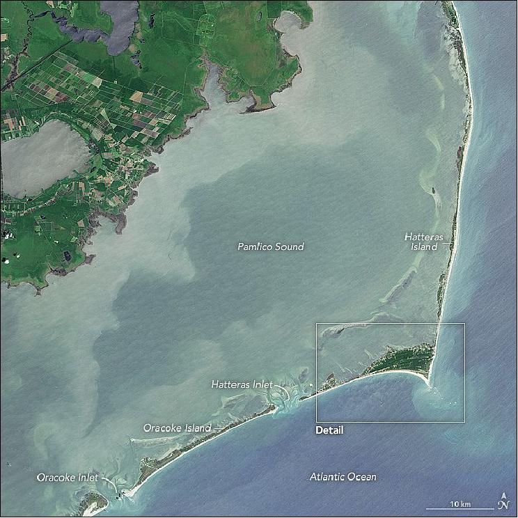
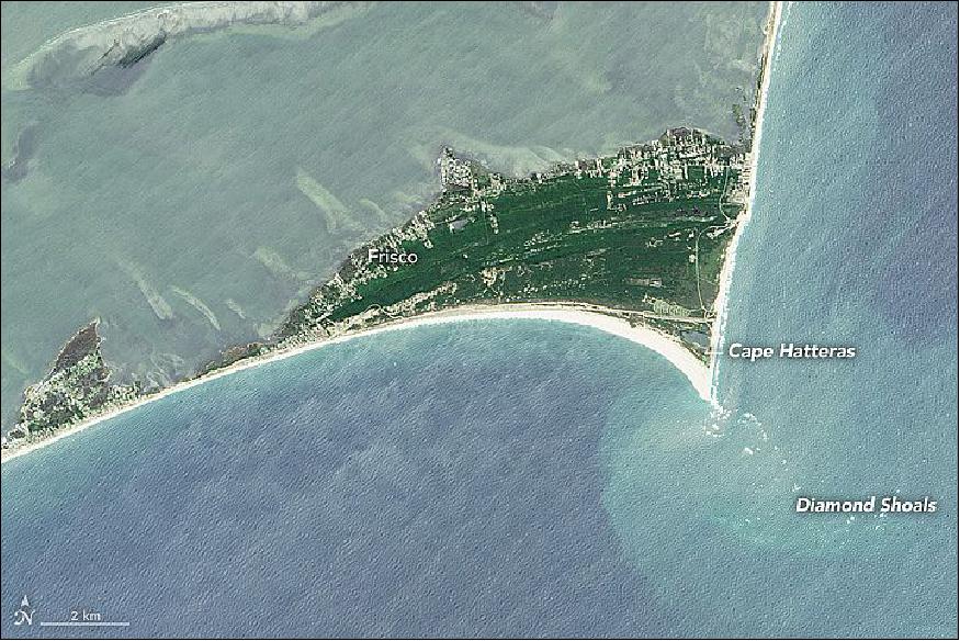
• July 4, 2016: The Greater Boston area, encompassing the eastern third of Massachusetts, is a playground for the American history enthusiast. Sites important to the American Revolutionary War are interspersed throughout the modern-day metropolitan region; the view from space shows how preserved historic landscapes coexist with the new (Figures 71 and 72). 56)
- In December 1773, American colonists protested British taxation and regulation by dumping hundreds of chests of tea overboard from merchant ships into Boston Harbor. The series of events that followed—including the march of British troops westward to confiscate a cache of weapons—culminated in battles in the towns of Lexington and Concord. The battles marked the start of the Revolutionary War in April 1775.
- The conflicts near Concord and Lexington are memorialized at Minute Man National Historical Park, shown in detail in the second image. By the 1950s, the area grew crowded with roads and suburban growth. Gas stations, restaurants, and an airfield all cropped up in an area that was once farmland and open fields. The park was established in 1959 in part to protect the historic landscape from further development.
- Route 2A cuts through the park and Hanscomb Field still stands as a nearby reminder of 20th Century modernization. In 2003, the National Trust for Historic Preservation listed Minute Man National Historical Park and nearby historic sites as one of the 11 most endangered historical places in the United States.
- Steps have been taken to restore historic structures and to return the landscape to one that more closely resembles the look and feel of the 18th century. For example, many power lines have been removed; stone walls have been rebuilt; and agricultural fields have been opened up. In 2009, the park boundaries grew to include the now-restored Barrett House and its surrounding farm, an important landmark of the war.
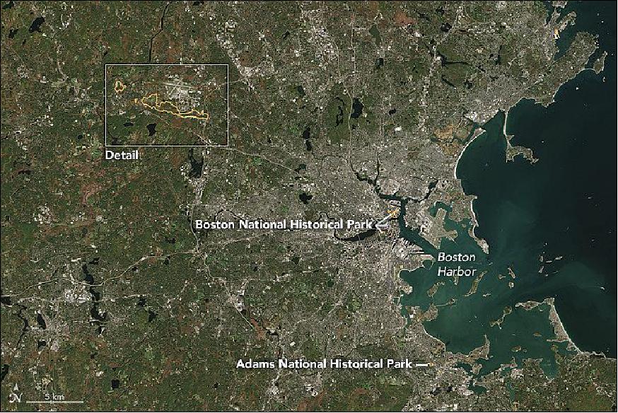
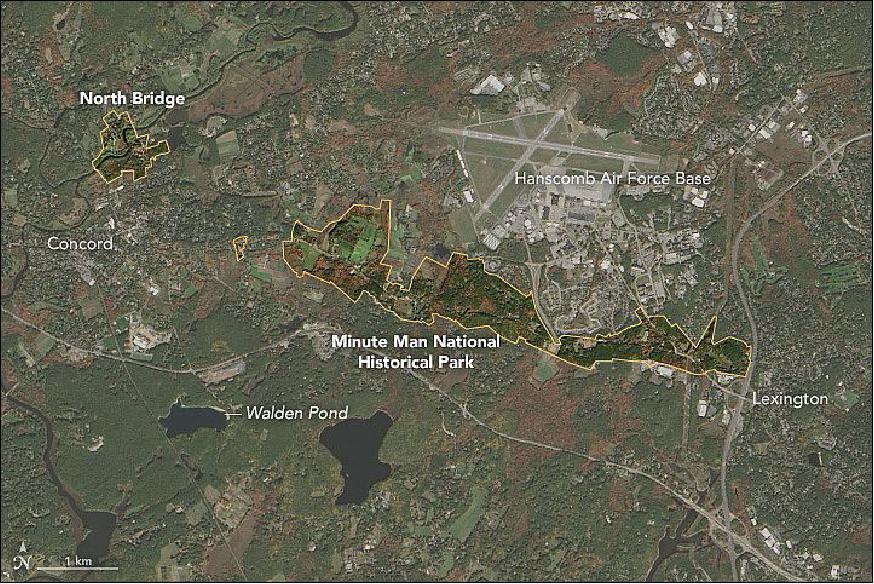
• June 15, 2016: Glacial Change in Montana's Blackfoot-Jackson Basin is shown in two Landsat images of 1984 and of 2015. At the current rate of glacier melting, a study arrived at the year 2030, in which the Montana's Glacier National Park will likely be glacier-free. 57)
- Scientists arrived at the year 2030 through a simple geospatial model running on software from the 1990s. The model depicted the change expected to occur to glaciers in the Blackfoot-Jackson basin (shown above), an area that contains the largest concentration of glaciers in Glacier National Park. At the time of the study, glaciers in the basin were also among the park's largest. "It was conjectured that if the largest glaciers disappeared by 2030, most of the smaller ones would probably disappear too," said Daniel Fagre, a research ecologist for the Northern Rocky Mountain Science Center of the U.S. Geological Survey.
- The model took into account the basic parameters, such as warmer summer temperatures and meteorological snowfall. It did not account for more complicated factors such as "snow avalanching" and "snow scouring"—things that can keep a small glacier alive. But despite its simplicity, the model painted an accurate, if broad, picture of the situation: the shrinking of the ice in Glacier National Park is real and happening fast. " People focus too much on the date, but the basic story is still true," Fagre said. "These glaciers will be more or less gone in the next several decades."
- Before these images were acquired, glaciers in the basin had already decreased from 21.6 km2 in area in 1850 to just 7.4km2 in 1979. The Blackfoot and Jackson glaciers once ran together, as a photograph from 1914 shows; by 2009, they had retreated into separate valleys.
- Other phenomena have left their mark on the landscape. In the 2015 image, a burn scar from the Thompson fire is visible southeast of Blackfoot glacier. As global and regional climate continues to warm, the frequency of fire in the park could increase.
- For now, the clearest reflection of climate change is the ice. Year-to-year weather variations matter somewhat, but most of the loss is a response to decadal trends in warming. As we approach 2030, most of these glaciers will be "small insignificant lumps of ice on the landscape," Fagre said. "These tiny remnants could last 10 to 15 years past that time if they are in sheltered places, but the park will no longer really have viable glaciers."
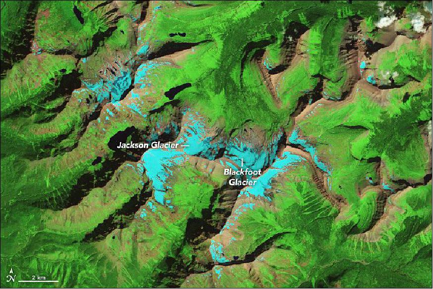
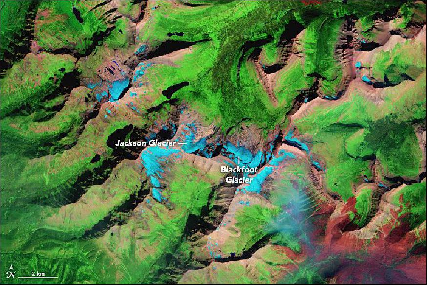
• May 31, 2016: The Rio Grande is a major North American river, flowing more than 3,000 km from Colorado to the Gulf of Mexico. In 1978, the U.S. Congress designated 315 km of the river along the U.S.-Mexico border as a "wild and scenic river." The designation protects the river's ecosystem and its natural free-flowing state. 58)
- Along the 134 km of the Lower Canyons area, you will find yourself in a truly remote river wilderness. This remoteness is likely part of the reason that a relatively small number of people visit the area compared to other sites managed by the National Park Service. Paddlers visit the Lower Canyons of the Rio Grande take advantage of this free-flowing river, maneuvering water ranging from calm to rapid as they float between canyon walls rising up 150 to 450 m. But it can take at least five days to emerge from a paddling trip through this part of the river.
- Despite its remoteness, the river is not immune from human influence. Dams upstream can affect the river downstream, changing the natural flooding cycles that normally shape the banks and build habitat for plants and animals. Drought can also affect the Rio Grande. In 2003 and 2015, portions of the river near El Paso ran dry.
• May 2016: Preparation for Emergency Conjunction Avoidance Maneuvers: The Landsat FOT (Flight Operations Team) has developed an E-RMM (Emergency -Risk Mitigation Maneuver) procedure, a combination of quick-build spacecraft command buffers and computer scripts, using specifically-defined and human-readable formats, to allow an engineering team the ability to quickly perform complex, critical spacecraft operations. 59)
- So far, Landsat-8 has been collecting nearly 75% more science images per day than originally designed, improving the cost-benefit ratio and expanding science coverage to nearly every day-lit opportunity through most of the year.
- The improved science collection tempo is enabled largely by the use of small, general-purpose command buffers in spacecraft flight software, called ROS (Relative Operations Sequences). ROS files (also called binaries, loads, or buffers), are small, temporary computer files containing a series of commands separated by defined delays, so that a single command can start the buffer and its contents will execute in a set order with predictable timing.
- The ROS loads can be built quickly and easily on the ground for any purpose, and one or more can be uplinked on each spacecraft contact as necessary. The addition of a special ground software script that begins the load process onboard at a specific time also allows the relative timing of the commands to be matched to wall clock times for precise execution of these buffers. Currently, ROS buffers are used for spacecraft science recorder file maintenance, automatically resetting balky equipment, and certain types of troubleshooting and fault recovery.
- The original operations concept at launch was to anticipate the need for a burn at the earliest warning, monitor until a few days before TCA (Time of Closest Approach), and evaluate the need for a burn around two days ahead of the Julian day when it would be executed, though the specific commit time was driven by the conjunction geometry and the TCA relative to the change of Julian day. A general spacecraft command load would be purpose-built to include the burn activities, including suspending science collections for the duration, and when uplinked we would be committed to performing at least part of the burn activities and losing the science collections. In preparing this early, we also committed to using best-guess information about the ΔV requirement; future changes to the ΔV would involve manual commanding and the risk of sending incorrect values.
- As ROS buffers became more widely used in day-to-day operations, a new process was developed to quickly build a special-purpose, propulsive-maneuver command sequence that could be used to avoid orbital debris. The burn concept was termed an Emergency Risk Mitigation Maneuver (E-RMM); it allows the burn to take place as soon as the new orbit can be screened for other conjunctions, instead of waiting for a new spacecraft command load to be built, and therefore provides a more responsive solution in a severely restrictive timeline. The special-purpose buffer includes all the commands the FOT normally inserts into the load for a standard orbit adjust maneuver (e.g., enabling burn software, setting thruster on-time duration, and so on) that can be uplinked, changed, rebuilt, and re-uplinked several times if necessary, and that could be started or stopped with minimal impact to the science imaging schedule. This buffer is built using a special computer script that takes in "knowledge" of when the buffer will start and codes in appropriate delays so that, once the buffer is started at the planned time, key events will happen at the desired wall clock time.
- As a result, FOT can plan and re-plan a burn quickly, uplink and execute the ROS buffer in a single contact, and reduce the time and uncertainty of burn planning from several days to around six hours. The use of a buffer that runs independently of the spacecraft's main command load also offers the ability to work around change-of-day and change-of-year boundaries; a clean break in science data collection from which the FOT can easily recover; and the ability to verify burn parameters quickly, maximizing the abort window.
- As of spring 2016, the Landsat-8 FOT has executed two demonstration burns and a DMU (Drag Make-Up) using E-RMM products. Though we have not executed an actual E-RMM burn on-orbit using this process, our ability to do so has saved team workload and science data collection on at least six occasions through the ability to wait and see how the conjunction event develops. As the low-earth orbit regime will continue to be polluted by space debris for the foreseeable future, the flexibility of burning correctly, and only when necessary, will provide significant benefits to cost, risk, and science for Landsat-8 and its successors.
• May 10, 2016: If a volcano erupts and there is no one there to see it, did it really erupt? Before the advent of satellites and seismic monitoring, volcanic eruptions in distant places would mostly go unnoticed unless they were absolutely extraordinary. Today, scientists can pick up signatures of events occurring far from any human observers.
- That was the case in late April and early May 2016 when satellite sensors detected signs of a volcanic eruption in the far South Atlantic Ocean between South America and Antarctica. Mount Sourabaya, a stratovolcano on Bristol Island, appeared to be erupting for the first time in 60 years. There are no human residents of the island, which is almost always covered in glacial ice and snow. 60)
- OLI (Operational Land Imager) on Landsat-8 acquired the Bristol Island image of Figure 76 using a combination of shortwave-infrared, near-infrared, and red light (Landsat bands 6-5-4) that helps detect the heat signatures of an eruption. The image shows the heat signatures (red-orange) of what is likely hot lava, while white plumes trail away from the crater. The band combination makes the ice cover of the island appear bright blue-green.
- With a roughly rectangular shape of 12 x 14 km, Bristol Island is one of the largest in the South Sandwich Islands chain. The highest peak on the island stands 1100 m above sea level. Due to the remote location and the lack of landing sites amidst its ice cap, the stratovolcano is one of the least studied in the world. The last known eruption on Bristol Island was reported in 1956.
• April 30, 2016: A key shipping route through Egypt recently received a major overhaul. The Suez Canal—the first artificial waterway connecting the Mediterranean Sea and the Red Sea—initially opened in November 1869 after 10 years of construction. The "New Suez Canal" opened in 2015 after just one year of construction. 61)
- Since its inception, the canal has been an economically important shortcut between Europe and Asia. The passage through Egypt meant cargo ships no longer had to sail around the southern tip of Africa. Expansion projects over the decades have helped the canal accommodate more traffic and larger ship sizes. The latest effort not only widened and deepened areas along the existing canal, it also added a 35 km new canal that runs parallel to the old one.
- The older single-lane canal, including the north and south access channels, spans 193 km from Port Said on the Mediterranean Sea to the Port of Suez on the Red Sea. Follow the canal south about 76 km from Port Said, and you reach the city of Ismailia, centered in these images. At km 95 you reach Great Bitter Lake, visible at the bottom of these images. The lake is one of the canal's designated holding and passing areas. The time spent waiting in these bypass areas was eased with the addition of the new parallel canal, visible in the right image.
• April 12, 2016: Toward the end of April, reprocessing efforts will begin for Landsat-8 OLI/TIRS scenes acquired from January 1 to March 31, 2016 along with data acquired during April, to create nominal Level-1 products containing valid TIRS data. Additionally, all future Landsat-8 scenes will contain valid TIRS data—however, newly processed data will use preliminary estimated position information from the TIRS SSM (Scene Select Mirror). 62)
- To compensate for not having TIRS SSM encoder information to indicate where the TIRS sensor is pointing, a new algorithm has been developed to provide estimates for the TIRS SSM encoder position. Note: SSM is also referred to as "Scene Select Mechanism".
• April 6, 2016: In the early 1600s, the English established their first permanent settlements in North America at Jamestown, Virginia, and then Plymouth, Massachusetts. But those were not the first attempts to colonize America. In the late 16th century, settlers started a settlement on Roanoke Island, North Carolina. The disappearance of that colony remains a mystery today. 63)
- On June 7, 2015, OLI (Operational Land Imager) on Landsat-8 captured this natural-color image of the northern half of Roanoke Island, which is tucked between North Carolina's mainland and barrier islands. Fort Raleigh National Historic Site, which was established 75 years ago on the island's northern shore, spans aquatic habitats, swamp forests, and a rare maritime evergreen forest. Fort Raleigh also preserves relics of England's first attempts to colonize the New World, as well as the history Native Americans, European Americans, and African Americans on Roanoke Island.
- The events that took place within the boundaries of the historic site are subject to debate. Initially, archaeologists thought that the northern part of the island was the main settlement of more than 100 English colonists who arrived in 1587. They based their claim on some European artifacts found within the historic site. But the artifacts were not indicative of habitation, and some experts speculate that the main settlement and fort were located farther south near Shallowbag Bay. Here, ships would be sheltered and settlers could more easily offload supplies.
- In any case, the island's entire settlement was found deserted in 1590. The story of the so-called "Lost Colony," as interpreted by playwright Paul Green, has been performed since 1937 at Fort Raleigh's beachfront theater, visible as a small tan fleck near the shoreline. Researchers have theorized that some of the settlers relocated about 80 km south to Hatteras Island. Other clues uncovered in 2012 from an old map suggest that some colonists might have ventured inland.
- At Fort Raleigh, one can also learn about the culture of the Algonquians, the natives who long inhabited the area, cultivated the land, and fished in the sounds long before Europeans arrived. Or read about a colony established centuries later during the Civil War, when more than 1,000 people—former slaves and families—found refuge on Roanoke.
• March 30, 2016: Just 25 km northwest of downtown Atlanta, a long parcel of undeveloped forests and hills cuts through the metropolitan suburbs (Figure 80). But the site was not always so peaceful. During the summer of 1864, the 2,965 acres (1,200 hectare) of this Civil War-oriented national park teemed with tens of thousands of men, horses, and cannons. 64)
- The hilly terrain played a role in the battle that commenced on June 27, 1864. Confederate forces had established an arc-shaped line that included Kennesaw Mountain, Little Kennesaw Mountain, Pigeon Hill, and areas to the south. A head-on attack by Union forces failed, and thousands of soldiers were killed. Park visitors can still see historical features, such as trenches that were dug for infantry and cannons. The defeat, however, was not enough to stop Union troops from advancing toward Atlanta, cutting off railroad supply lines, and ultimately reaching the city in early September 1864.
- As this satellite view shows, the mountain ridge is a major geographic feature of the area. Steep, rocky slopes of the range rise on average to about 550 m above sea level. Outcrops and boulders are scattered among a mostly forested landscape. The image was acquired in winter, so vegetation appears less lush and green than it would in summer, when the deciduous trees have foliage. Still, historical surveys note that the landscape during the Civil War battle was even barer, as the summits had been cleared of trees.
- Today, heavy urbanization—roadways and private residential housing—surrounds the park. Construction around the battlefield put additional pressure on the park, which stands as the largest free park in the heavily developed Atlanta metropolitan area. Park managers have had to balance preservation of the memorial landscape with the needs of nearby residents who use the space for recreation and as a commuting route.
• March 20, 2016: It's an archetypal American story: grandeur and legend rising from modest, humble beginnings. Both islands (Figure 81) were once home to vast oyster beds, and one was built up from the spoilings and fill from nearby dredging operations. Then in the late 19th century, the two islands became central to the narrative of the United States of America as "melting pot" for different cultures and a beacon of hope for the "tired, poor, huddled masses" of the world looking to make a new start. 65)
- Liberty Island, once known Bedloe's Island, was an oyster harvesting ground for the Lenape Indians and later for early European settlers. It then saw stints as a quarantine station, a hospital, and a military outpost. Fort Wood, with its walls shaped into an eleven-point star, eventually became the foundation for the Statue of Liberty, which was completed in 1886. The statue was designated a national monument in 1924, and in 1933 responsibility for the statue and island was transferred to the National Park Service. Today Liberty Island is one of the most visited sites in the National Park system, with nearly 4.3 million visitors per year.
- Ellis Island has long had a complicated relationship with the "New Colossus" standing next door. Many people referred to it as the "Island of Hope, Island of Tears." From 1882 to 1954, more than 12 million new immigrants to the United States made their entry to the country through the processing station on Ellis Island. The busiest year was 1907, when 1,004,756 immigrants were processed — 11,747 of them on April 17, the busiest day.
• March 15, 2016: ESA has agreed with NASA, NOAA and the USGS to make data available to them from the European Sentinel satellites. With the third Copernicus satellite, Sentinel-3A, recently launched, ESA has signed technical arrangements with these US agencies for accessing Sentinel data. These arrangements coordinate the technical implementation covering the Sentinel data access to the US. 66) 67)
- ESA and its international partners are pursuing Earth observation activities in a number of areas of common interest, and are sharing each other's satellite data. All sides are committed to the principle of full, free and open access to the European Sentinel and the NASA, NOAA and USGS Earth observation satellite data and information.
- The signed arrangement will allow NASA, NOAA and USGS to systematically retrieve the Sentinel data from a dedicated International Data Hub operated by ESA. These agencies will then transfer the data to the US, absorbing them in their existing data access systems, such as EarthExplorer and GloVIS, and disseminating them to their own user communities.
- For over three decades, ESA has been acquiring, processing and disseminating data from a number of US missions such as Landsat to the European user communities as part of its Earthnet Third Party Mission Program.
- While the US agencies' objective is to serve the US user communities with priority, the Sentinel data will continue to be freely accessible for Copernicus Services, as well as to users worldwide, through the ESA operated data hubs.
• March 13, 2016: In February 2016, the United States government established the world's second-largest desert preserve. In designating three new national monuments in the California desert, the U.S. DOI (Department of the Interior) added 1.8 million acres (728, 400 hectare) to an existing 7.6 million acres (3, 075, 600 hectare) of protected land. This image from the Operational Land Imager (OLI) on Landsat 8 shows how they all connect. (The image is a composite of satellite data from Landsat 8 passes on February 8 and February 17, 2016.). 68)
- The western edge of Sand to Snow National Monument is located about 120 km east of downtown Los Angeles. This aptly named monument encompasses 150,000 acres (60,700 hectare) from the floor of the Sonoran Desert to the mountaintops in San Bernardino National Forest. Ecological diversity at the various altitudes makes this monument unique.
- Hikers encounter some of this diversity along 50 km of the Pacific Crest Trail that crosses through the monument, from Whitewater Canyon up 2100 m to Mission Springs.
- Sand to Snow shares a common boundary with Joshua Tree National Park, which in turn connects to Mojave Trails National Monument—the largest new addition at 1.6 million acres. Lava flows and mountains spread across this tract of the Mojave Desert. The focal point is the sand dunes; in particular, the remote and nearly pristine Cadiz Dunes that formed from the sand of dry lake beds.
- Finally, tucked into the northeast corner of the pre-existing Mojave National Preserve is the smallest addition—the 20,920 acres (8,460 hectare) of Castle Mountains National Monument. But this smallest addition is an important one. Inclusion of Castle Mountains connects ecosystems in the New York Mountains and the Piute Mountains. Protection of this area ensures that habitat stays intact for wildlife such as the desert bighorn sheep.
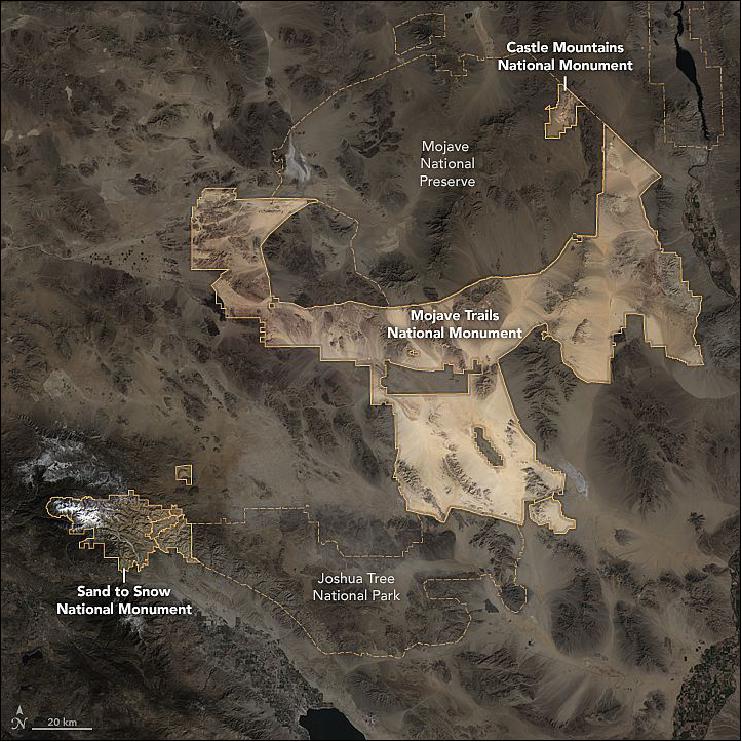
• Feb. 18, 2016: A partnership has been established between ESA (European Space Agency) and the USGS to allow for USGS storage and redistribution of data acquired by the MSI (Multispectral Instrument) on ESA's Sentinel-2A satellite that was launched in June 2015. The collaborative effort between ESA and USGS will provide for public access and redistribution of global acquisitions of Sentinel-2A data at no cost, allowing users to download the MSI imagery from the USGS. The MSI sensor acquires 13 spectral bands that are highly complementary to data acquired by the USGS Landsat-8 OLI (Operational Land Imager) and Landsat 7 ETM+ (Enhanced Thematic Mapper Plus). 69)
• Feb. 11, 2016: Today the Landsat-8 spacecraft is 3 year on orbit and operational. So far, the satellite has acquired more than 675,000 scenes, adding valuable time series data to the USGS Landsat Archives!
- As of February 10, 2016, many of the scenes acquired from October to December 2015 have been reprocessed into nominal Level-1 products containing valid TIRS (Thermal Infrared Sensor) data and are available for download. The generation of Landsat-8 surface reflectance products from these data will become available within the next week. 70)
• January 26, 2016: Two days after a massive winter storm system dropped snow from Tennessee and Georgia to Massachusetts, millions of Americans are digging out. By some news accounts, more than 30 million people lived in areas that received at least 50 cm of snow, and 3 million more saw at least 75 cm. 71)
- The highest snow total was recorded in Glengarry, West Virginia at 107 cm. Snow totals approached records at airports near Baltimore at 74 cm, Philadelphia at 57 cm, and Newark, New Jersey at 71 cm. The National Zoo in Washington, D.C. counted 57 cm and Central Park in New York picked up 68 cm.
- At least 37 people have died as a result of car accidents, hypothermia, carbon monoxide poisoning, or over-exertion from shoveling snow, according to multiple news reports. At least a quarter-million people have lost electric power, and more than 13,000 airline flights have been canceled.
- Beyond the snowfall, near-hurricane force winds combined with astronomically high tides to produce storm surges on the Delaware and New Jersey coasts. Sea water poured into coastal towns, while extensive beach erosion occurred as far north as Massachusetts.
• January 13, 2016: The Landsat-8 TIRS (Thermal Infrared Sensor) data continue to be collected with the scene select mirror encoder electronics disabled (mode 0). While in this mode, the TIRS LOS (Line of Sight) model will be regularly updated and modifications are being made to automate revisions to the LOS in the LPGS (Level-1 Product Generation System). 72)
- OLI and TIRS data that have been collected through the 4th quarter of 2015 (October-December); they will be reprocessed into nominal Level-1 products containing valid TIRS data, and will be available in February 2016.
- TIRS data acquired during the 1st quarter of 2016 (January-March) will be reprocessed and made available in April 2016. A strategy is being developed for generating near-realtime products moving forward while operating in mode 0. More details will be posted on the Landsat Missions Web site as they become available.
• Nov. 17, 2015: The Landsat-8 FOT (Flight Operations Team) continues to monitor current levels within TIRS (Thermal Infrared Sensor) SSM (Scene Select Mirror) encoder electronics. The FOT and Calibration Validation team are continuing to investigate the current anomaly and analyze instrument telemetry data in order to accurately measure the position of the SSM and to develop the necessary parameters for the processing TIRS data under an alternative operations concept. 73)
- TIRS data will continue to be routinely collected but will not be processed to Level-1 products until the geometric model parameters are finalized and the algorithms and code in the LPGS (Landsat Level-1 Product Generation System) have been updated, tested, and verified. These activities are expected to be completed no sooner than February 2016, at which time all products will be reprocessed to provide valid TIRS data.
- Following the implementation of an alternate TIRS processing capability, the zero-fill Landsat-8 scenes will be reprocessed and made available from the USGS archive. Mission operations will continually assess potential opportunities for return to normal operations on the B-side encoder electronics. However, at this time, the probability of return to normal operations is unknown.
• Nov. 13, 2015: Free Data Proves Its Worth for Observing Earth. Since late 2008, when Landsat Earth observation images were made available to all users free of charge, nearly 30 million Landsat scenes have been downloaded through the USGS (U.S. Geological Survey) portal – and the rate of downloads is still increasing. That's a lot of free data about the state of the planet. But what is it worth? How valuable can something free possibly be? 74)
- The worth of many things is related to scarcity. If there are too many houses or diamonds, bushels of corn or barrels of oil for sale, the price for these items falls. A free market determines the market value of what we might hope is a $500,000 house or a $5,000 diamond.
- The concept of market value breaks down for goods and services that society has determined should be freely available to everyone. Free data for earth observation fits into this category. It is a public good – along with public education, public roads, and public parks. While these services are not actually free (they are, of course, funded with public money), we know that the broad use of such services benefits all of society so the cost to each individual user is largely borne by all.
- The Department of the Interior's policy of releasing the full Landsat archive at no cost allows researchers around the world in government, in the private sector, and at universities and institutions to generate even more data applications that are good for society. These purpose-driven data applications – known on mobile devices as "data apps" – can serve commercial endeavors in agriculture and forestry; they can enable land managers in and out of government to work more efficiently; they can help us define and address critical climate and environmental issues.
- The DOI (Department of the Interior) policy of releasing the full Landsat archive at no cost allows researchers around the world in government, in the private sector, and at universities and institutions to generate even more data applications that are good for society. These purpose-driven data applications – known on mobile devices as "data apps" – can serve commercial endeavors in agriculture and forestry; they can enable land managers in and out of government to work more efficiently; they can help us define and address critical climate and environmental issues.
- In the United States, the federal government invests about $3.5 billion annually in civil earth observations and data (including Landsat and other satellites, weather, GPS, etc.) across multiple agencies, while optimizing related investments that are also made by state, local and tribal governments, academia, and industry. The information derived from earth observations supplies the foundation for scientific advances in many fields and enables multiple federal agencies and partners to carry out their missions. Federal investments in various aspects of earth observation are conservatively estimated to add $30 billion to the U.S. economy each year by providing Americans with critical knowledge about natural resources, climate and weather, disaster events, land-use change, ecosystem health, ocean trends, and many other earth-related phenomena.
- The USGS, a bureau of the DOI, is a major contributor to civilian earth observation through its support of the Landsat mission in partnership with NASA. First launched by NASA in 1972, the Landsat series of satellites has produced the longest, continuous record of Earth's land surface as seen from space.
- Landsat images spanning four decades have been used by scientists and resource managers to monitor water quality, glacier recession, coral reef health, land use change, deforestation rates, and population growth. To give a few examples of Landsat's many commercial applications, Landsat data have been used to track the use of irrigation water, to assist drought-stricken California grape growers, and to contribute to the success of a forestry start-up company. As an indication of widespread public interest in Landsat data, third party avenues to the data and innovative ways to use it are available from Amazon, ESRI (Environmental Systems Research Institute) and Google.
- A recent White House-led assessment determined that Landsat is among the Nation's most critical Earth observing systems, second only to GPS and weather. In 2013, the U.S. National Research Council found, "The economic and scientific benefits to the United States of Landsat imagery far exceed the investment in the system." In 2014, the Landsat Advisory Group of the National Geospatial Advisory Committee was as even more specific in its finding, "The economic value of just one year of Landsat data far exceeds the multi-year total cost of building, launching, and managing Landsat satellites and sensors."
- Other nations recognize the benefits of free and open data. Fundamental knowledge of the land and its resources is a basic need for effective government and a productive economy in any nation. More than 30 countries and geopolitical groups now have earth observing satellites, reflecting a wide range of national priorities around the world for environmental monitoring and economic growth. At the same time, more countries are adopting policies of full, free, and open data for earth observation, whether the observation operations are conducted by their national satellites or whether the data is shared between countries and with the public. — In Rwanda, for example, the government has developed and used open data to support national land use planning via their National Land Use Portal, which provides transparency collaboration and cooperation among many different partners to help shape a more sustainable future. Brazil, a co-leader of the Open Government Partnership in South America, provides its citizens the opportunity to participate in the planning and development of public policies by providing government data on hydrography, transportation, energy and communications, and more, through their Brazilian Portal of Open Data.
- October 19, 2015: The United States and the European Commission signed an agreement on Copernicus Cooperation. The European Copernicus Program has adopted a policy of free and open data from its Sentinel series of satellite missions, helping make Europe a world leader in the implementation of free and open data policies. U.S. Deputy Assistant Secretary of State for Science, Space and Health Jonathan Margolis and European Commission Director for Space Policy, Copernicus and Defence Philippe Brunet signed the arrangement in Washington, D.C., on October 16. The arrangement will allow experts from U.S. agencies, including NASA, NOAA, and the USGS, to pursue cooperative data sharing activities with European counterparts, including the European Commission,ESA (European Space Agency), and EUMETSAT (European Organization for the Exploitation of Meteorological Satellites). This cooperation will enhance data access, validation, and quality control as well as satellite system compatibility, interoperability, and instrument inter-calibration. 75)
• In October 2015, a system of storms caused significant flooding in most of California's Death Valley National Park. Flash floods from the storm destroyed roads and utilities, and damaged several historical structures. In particular, a flash flood of water and mud caused extensive damage to Scotty's Castle, an ornate mansion built in the 1930s and one of the most popular landmarks in Death Valley National Park. The Oct. 18-19 storm dumped ~7 cm of rain, more than the region typically gets in a year. 76)
• August 12, 2015: Algae are complicated. The little plants can be both good and bad. Single-celled algae called phytoplankton are a main source of food for fish and other aquatic life, and account for half of the photosynthetic activity on Earth—that's good. 77) 78)
- But certain varieties such as some cyanobacteria produce toxins that can harm humans, fish, and other animals. Under certain conditions, algae populations can grow explosively — a spectacle known as an algal bloom, which can cover hundreds of square kilometers. For example, in August 2014, a cyanobacteria outbreak in Lake Erie prompted Toledo, Ohio, officials to ban the use of drinking water supplied to more than 400,000 residents. - In the United States alone, freshwater degradation from "bad" algae costs the economy about $64 million a year.
- NASA, the U.S. EPA (Environmental Protection Agency), NOAA (National Oceanic and Atmospheric Administration), and the USGS (U.S. Geological Survey) are doing something about it. NASA has long used Earth observing satellites to locate algal bloom outbreaks in the ocean. But now, this unique satellite data will be routinely produced in a form that helps US water quality managers monitor the freshwater. Water quality managers will soon, with a peek at their cell phones, have an answer to "how's the water?"
- The four agencies are working on a joint project, sponsored by NASA, to transform satellite data into an indicator of cyanobacteria outbreaks in the freshwater supply. The data will be integrated into an EPA Android smart phone application so environmental officials can see – at a glance – the condition of a specific water body.
- "With our app, you can view water quality on the scale of the US, and zoom in to get near-real-time data for a local lake," explains the EPA's Blake Schaeffer, Principal Investigator for the project. "When we start pushing this data to smartphone apps, we will have achieved something that's never been done – provide water quality satellite data like weather data. People will be able to check the amount of ‘algae bloom' like they would check the temperature."
- Here's how it works: A harmful species of cyanobacteria emits chlorophyll and fluorescent light at various points in their life cycles. Landsat and NASA's MODIS (Moderate Resolution Imaging Spectroradiometer ) can detect these "ocean color" signals, which reveal the location and abundance of cyanobacteria. The project team will collect this data for freshwater bodies and convert it into a form accessible through web portals and the EPA mobile app. In addition to MODIS, they'll draw data from the Sentinel-2 and Sentinel-3 satellites of ESA (European Space Agency).
- With early warning about a developing bloom, officials at water treatment plants will be better able to determine when, where, and how much to treat the water to keep consumers safe. That means unnecessary — and expensive — overtreatment may be avoided. The data will also help park managers alert swimmers, boaters, and other recreational users to hazardous conditions. Says NASA Administrator Charles Bolden: "We're excited to be putting NASA's expertise in space and scientific exploration to work protecting public health and safety."
- The project will also help scientists understand why "bad" algae outbreaks occur. By comparing the color data with landcover change data, they'll learn more about environmental factors that spur algal growth. The result: better forecasts of bloom events. So we'll know when an algae bloom is safe or harmful.
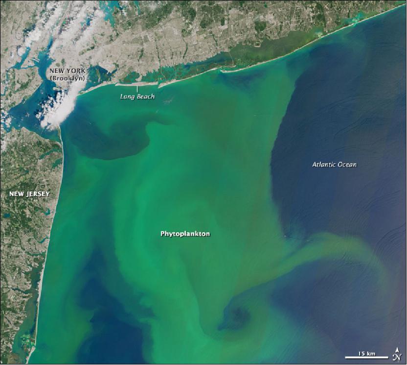
• July 17, 2015: Located near the western edge of the Sahara Desert, the Eye of the Sahara is a feature that resembles a large eye when viewed from space. Also known as the Richat Structure or Guelb er Richat, the Eye is a symmetrical dome of eroded sedimentary and volcanic rock. The outermost rings measure approximately 40 km across. Persistent northeasterly winds keep much of the dome free from sand, exposing the various layers of rock. The circular feature was initially interpreted to be an asteroid impact structure, but most scientists have now concluded that it was caused by geologic uplift. 79)
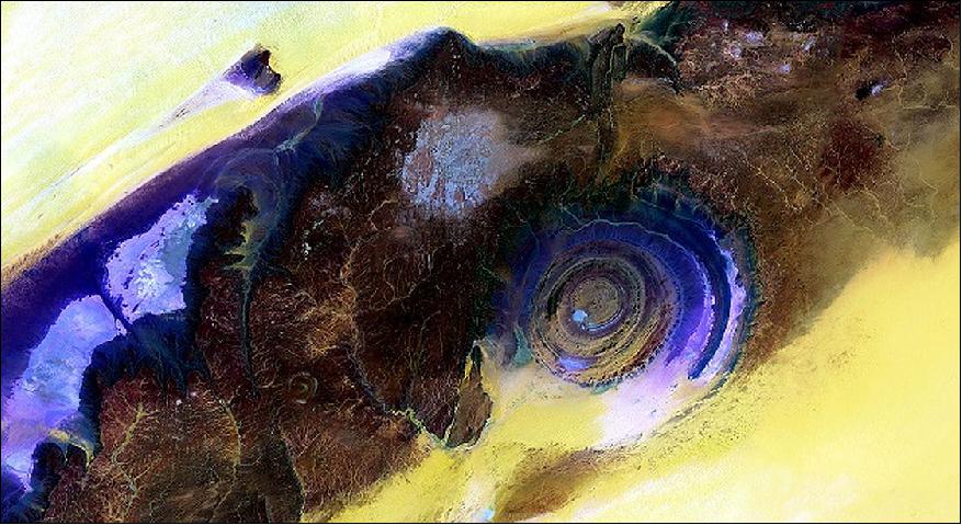
• June 19, 2015: The Landsat-8 image of the San Francisco Bay Area (Figure 88) was released by ESA in the 'Earth from Space video program'. The city of San Francisco is on a peninsula in the center left section of the image. In the upper-central portion, we can see the delta of the Sacramento and San Joaquin rivers with brown, sediment-filled water flowing down into the larger bay. Starting in the top-left corner of the image and running diagonally to the south is the San Andreas Fault. This is the border between the North American and the Pacific tectonic plates, and is responsible for the high earthquake risk in the area. 80)
Surrounding the Bay one can see densely populated urban areas in white/grey, while forests and park areas appear in shades of green. In the upper-right corner, one can see geometric shapes of large-scale agriculture, with fields in different colors depending on the vegetation type. Distinguishing between different types of land cover is an important task for Earth-observing satellites, helping us to understand the landscape, map how it is used and monitor changes over time.
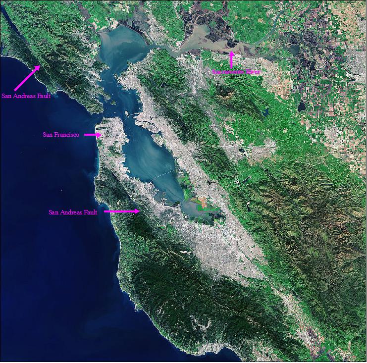
• July 7, 2015: The Landsat-8 spacecraft and its subsystems are operating nominally. 81)
TIRS anomaly: • 19 Dec. 2014 – Mechanical Control Electronics (MCE) reached a yellow over-current limit. Scene Select Mirror (SSM) encoder was switched to ‘Mode-0' which basically disables the encoder - TIRS bands in products were set to 0 (until we reprocess to handle mirror drift) • 2 Mar. 2015 – TIRS switched to Side-B ‘Mode-4'. Commission and calibration period followed - Develop new parameters for CPF, BPF, RLUT • 30 Apr. 2015 – Reprocessing of TIRS data started - Mode-0 data (19 Dec. 2014 – 2 Mar. 2015) - Commissioning data – Side-B ‘Mode-4' data (2 Mar. 2015 – 30 Apr. 2015) • 14 May 2015 – Reprocessing completed. TIRS Stray Light: • Discussion forthcoming (Ron Morfitt) • Tentatively planned for LPGS 2.6 (~October) • Plan to reprocess OLI_TIRS data once stray light algorithm is validated |
• May 20, 2015: Since measurements began in 1895, Alaska's Hubbard Glacier has been thickening and steadily advancing into Disenchantment Bay. The advance runs counter to so many thinning and retreating glaciers nearby in Alaska and around the world. The image of Figure89 , acquired by OLI (Operational Land Imager) on Landsat-8, shows Hubbard Glacier on July 22, 2014. The yellow lines indicate the location of the terminus on August 1, 1978, and on July 13, 2002. - The image of Figure 90 shows a close-up of the glacier's terminus on July 13, 2002. 82)
- According to Leigh Stearns, a glaciologist at the University of Kansas, Hubbard's advance is due to its large accumulation area; the glacier's catchment basin extends far into the Saint Elias Mountains. Snow that falls into the basin either melts or flows down to the terminus, causing Hubbard to steadily grow. In addition, Hubbard is building up a large moraine, shoveling sediment, rock, and other debris from Earth's surface onto the glacier's leading edge. The moraine at the front gives the glacier stability and allows it to advance more easily because the ice does not need to be as thick to stay grounded. - If it is thin, it can start floating and will not necessarily advance.
- Twice in the past hundred years — in 1986 and again in 2002 — the moraine has made contact with Gilbert Point and blocked the entrance to Russell Fjord. With nowhere to drain, runoff caused the water level in the fjord to rise rapidly. Water levels to rose 0.24 m per day. However, the closure was temporary, as water pressure overpowered the encroaching ice and debris and burst through the natural dam, returning the fjord to normal levels.
- In 2002, Leigh Stearns was attending a glaciology conference in nearby Yakutat, Alaska, a town that depends on Russell Fjord's marine life. "Understanding Hubbard's behavior is scientifically interesting," Stearns said, "but it also has immediate consequences for the town of Yakutat." — Those consequences provoked her to investigate what controls the terminus position and its advance, and to estimate when the fjord might become permanently blocked. The findings, recently accepted for publication in the Journal of Geophysical Research, explain how the mechanics at the terminus override the influence of other climate fluctuations. 83)
- One estimate suggests that the fjord could permanently close by 2025. But Hubbard's terminus is nearly 14 km wide, and does not advance at the same rate across its entire width. The region adjacent to Gilbert Point, where the closure would occur, advances more slowly, because seawater passing through the gap constantly erodes the ice. Based on the current rate of advance at the gap, Leigh Stearns estimated that closure could occur by 2043. Leigh Stearns cautions, however, that these closure dates are "projections based on our current observations, and should be viewed with skepticism."
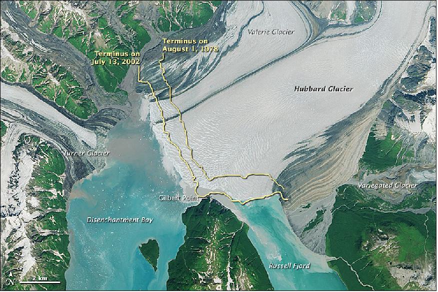
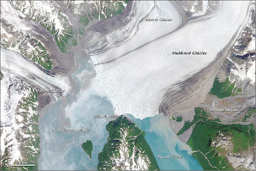
• May 8, 2015: On March 6, 2015 the Landsat-8 TIRS (Thermal Infrared Sensor) switched from A side to B side electronics to resolve a problem with the A side encoder electronics. At that time, a plan was outlined for reprocessing data acquired since the problem began. 84)
- Beginning April 30, 2015, Landsat-8 scenes acquired from December 19, 2014 to March 13, 2015 began reprocessing to repopulate the TIRS data in the products. This calibration notice details the data changes during this timeframe. The reprocessing effort is expected to complete by May 18, 2015.
- Some TIRS data for a number of scenes will not be processed due to non-nominal instrument configuration. There were several intervals identified that the data was good for a portion of the interval, but where the SSM (Scene Select Mechanism) was commanded to rotate off nadir making the TIRS data unusable for the other portion of the interval. The reprocessing will process those where TIRS was well outside the field of view of OLI due to an off nadir SSM as OLI only products.
• April 16, 2015: Landsat-8 Thermal Data Reprocessing Update. On March 6, 2015 , USGS reported that the Landsat-8 TIRS (Thermal Infrared Sensor) resumed normal imaging operations, and outlined plans for reprocessing data acquired since December 19, 2014, when problems occurred in the A-side electronics of the sensor. Provisional TIRS data acquired since March 13, 2015 were expected to require reprocessing to refine the absolute calibration; however, based on a small number of vicarious measurements, it has been determined that these data will not need to be reprocessed for now since the radiometry appears to be consistent with the previous A-side data. The calibration will be monitored and updated in the future if needed. 85)
• April 12, 2015: March 2015 marked the 15th year that iceberg B-15 remained afloat around Antarctica... at least what's left of it. The iceberg first made its break from the Ross Ice Shelf in late March 2000. One of the largest icebergs ever observed, it measured about 270 km long and 40 km wide — almost as large as the state of Connecticut. 86)
- Fifteen years later, the U.S. National Ice Center (NIC) reported that eight fragments of the original berg remain (icebergs and fragments must measure at least 19 km long in order to be named and tracked by the center). According to NIC's weekly report from April 3, 2015, the largest surviving fragment was B-15T, which measured 52 km long and 13 km wide.
- The OLI (Operational Land Imager) on Landsat-8 acquired this natural-color image of B-15T on January 14, 2015 (Figure 91). The iceberg was located amid sea ice off the Princess Astrid Coast, just east of its position pictured in an image acquired April 5, 2015, by the MODIS (Moderate Resolution Imaging Spectroradiometer) on NASA's Terra satellite.
- Many icebergs get caught up in the currents circling Antarctica and then eventually spin off to the north and break up. However, icebergs that stay trapped in cool coastal waters can persist for decades.
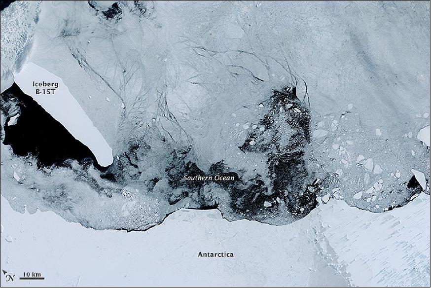
• March 25, 2015: Landsat is a key data input for many products developed and used in water resources, agricultural monitoring, land use and land cover monitoring, forest management, and development planning. Yet, Landsat's contribution goes beyond its use solely as a primary data input. The products and processes developed by the Landsat program provide tools for data accuracy and visual communication improvement of other satellite imagery. These products are provided by the Landsat program at no cost to the users and have proven to be valuable assets to the private tech sector. This case study explores that various correction capabilities that Landsat offers to other satellite operators, acting as a tool in improvement of usability of other imagery. Several satellite companies and satellite imagery users are highlighted as beneficiaries of Landsat products. | |
- Landsat base layer: A base layer is a data set used as a reference for the display, analysis or correction of other data. Imagery, such as from Landsat and Landsat-like satellites is often used as a base layer. As a base layer, Landsat imagery is particularly helpful for verifying the accuracy of data due to the high quality of geometric correction and orthorectification of Landsat Level 1T data. Frank Warmerdam of Planet Labs, a company that designs, builds and operates a network of small satellites, notes that Landsat's high quality scenes provide a "trusted global basemap" for public and private sector use. Mapbox (Mapbox with HQ in Washington DC is one of the biggest providers of custom online maps for major websites) creates custom maps with open source tools and uses Landsat imagery as a basemap for a wide range of moderate resolution products. DigitalGlobe, a satellite imagery provider, is another user of Landsat imagery. As DigitalGlobe's data archive continues to grow, their use of Landsat imagery will likely be declining. However, the company used Landsat imagery to get started with their "DigitalGlobe Basemap" product series. Landsat data are also used by DigitalGlobe in parts of the world where either no high resolution data or no recent high resolution data is available. | |
- Processing satellite data using Landsat: A vast amount of processing is required to take the raw imagery collected by satellites and translate it into usable data for analysis. Spatial and spectral corrections are necessary in order to accurately locate the imagery on the earth's surface and convert pixel values to meaningful measures of the surface being captured. The Landsat program offers state of the art technology and methodology for conducting these corrections and as a result provides trusted remotely sensed data set for global coverage at the moderate resolution level. Due to Landsat's high standards and well documented approaches to spatial and spectral corrections, the correction and calibration of other satellite imagery can be achieved through the use of Landsat imagery. | |
- Spatial correction: Spatial correction, sometimes referred to as geo-rectification, geo-registration or spatial tie-down, involves accurately locating imagery on the earth's surface as well as correcting for distortions in the image through geometric correction and orthorectification. Geometric correction requires assigning known coordinates to points in the image, which geolocates the image to the correct place on the Earth's surface. Additionally, it corrects for large scale distortion or error inherent in image due to earth movement, earth curvature, and/or satellite movement during collection. Correcting small scale distortion is done through orthorectification, a type of geometric correction that utilizes digital elevation data to more accurately correct for distortions due to terrain. The capability of Landsat to assist in spatial correction of other satellite data is utilized by companies such as DMCii, Planet Labs and BlackBridge. DMCii, a satellite imagery provider, uses Landsat data as a base layer for providing orthorectification for customers who do not have their own reference data, which is most of their customer base. This helps keep the costs down while improving the accuracy of DMCii's products. Planet Labs uses Landsat for the spatial tie down process everywhere around the globe for consistency and convenience. However, when processing difficult areas such as jungles and mountains, Landsat is a particularly critical resource. "Without Landsat it would be essentially impossible to get good GCP (Ground Control Point) locations from other sources," says Frank Warmerdam of Planet Labs. Similarly, BlackBridge, Canada's foremost supplier of satellite imagery products, is using Landsat imagery to perform geometric correction and orthorectification on areas in northern Africa and eastern Asia, where no better GCP's are available. BlackBridge has been using Landsat GCP since 2009 on about 750,000-800,000 out of 1 million products. The company will likely continue to use Landsat GCP's until higher accuracy GCP's become available for the rest of the landmass on Earth. | |
- Spectral corrections: Another important component of imagery processing is spectral correction. Spectral correction includes spectral characterization and radiometric calibration. Spectral characterization is a process of determining how different portions of the electromagnetic wavelength interact with an object. Radiometric calibration is a broader term for the process of relating values recorded (sensed) by a satellite sensor with radiance values (what was actually reflected/emitted on the ground). Calibration can either be absolute or relative and can employ different methods depending on when in the process the calibration is being performed. For radiometric calibration, cross-calibration and surface reflectance are the principle processes used to correct satellite imagery. Cross-calibration is a form of relative calibration which compares values collected by one satellite sensor against values collected by a second satellite sensor. If one of the sensors has had corrections applied, the corrected values can be used for relative radiometric calibration of the other sensor. This method can be a cost effective method for radiometric calibration of operational satellites (Liu et al. 2004). DMCii initially used Landsat 7 as a standard reference satellite for cross-calibration over Libya and Antarctica. The company is now working on incorporating Landsat 8 data, which produces a good long term baseline for cross-calibration. In the future, DMCii anticipates incorporating data from the European Union Sentinel-2 mission into their tool kit. For certain analyses of satellite imagery, it is necessary to calibrate for surface reflectance, which is the ratio of solar energy that is reflected rather than absorbed by an object on the earth's surface. However, the reflected energy must first pass back through the atmosphere before it is detected by the satellite sensor. As a result, corrections must be applied to remove atmospheric effects. Landsat currently uses a set of algorithms known as LEDAPS (Landsat Ecosystem Disturbance Adaptive Processing System ). This type of radiometric calibration uses auxiliary data including ozone, water vapor, geopotential height, and aerosol optical thickness to calculate surface reflectance. Once these corrections are applied, surface reflectance products represent what radiance values would be under ideal conditions (i.e., no atmospheric effects). Many higher-level surface geospatial analyses—including vegetation indexes, albedo, LAI (Leaf Area Index), burned area, land cover, and land cover change – rely on surface reflectance products. The availability of these products in the private sector is highly valued by the users. Mapbox reports that of all the atmospheric correction methods tested by them, LEDAPS is the one they trust most. "LEDAPS allows types of comparison and analyses that would otherwise require significant single-purpose investments. We estimate that LEDAPS has saved our company approximately $250,000 in technical and opportunity costs over the last 24 months, and that number is steadily increasing," says Charlie Loyd, a member of Mapbox's satellite team. "Other than its accuracy, the key to LEDAPS's value to us is its generality. We can apply LEDAPS to a Landsat scene once and have output that's equally appropriate for true color imagery, classification algorithms, NDVI (Normalized Difference Vegetation Index), and other indexes. We recommend it broadly, knowing that it will meet virtually any user's needs for atmospheric correction. For these reasons, LEDAPS is the only non–in-house component of our Landsat software pipelines that we consider effectively irreplaceable." DigitalGlobe is another company that has accrued benefits through LEDAPS. The company sees Landsat as a key input in the development process of their own surface reflectance product. In 2013, DigitalGlobe introduced a new product, seamless country-scale orthomosaics at half meter resolution, using Landsat for surface reflectance to bootstrap to a base map. DigitalGlobe reports that having Landsat data available accelerated the introduction of the product by about 9 months. While the company does not break out revenue by product in their public reporting, this particular product represents multiple millions of dollars of revenue annually. | |
- Additional benefits: In addition to the more specific spatial and spectral correction benefits discussed above, the Landsat program as a whole offers additional benefits to the private satellite imagery community. According to Frank Warmerdam of Planet Labs, the Landsat archive acts as a common reference point among datasets, where the well-published and respected nature of Landsat products provides a reference for product to product relation. Along with Landsat's long continuous data record and exceptional technical integrity, it is made indispensable by its free distribution (Charlie Loyd, Mapbox, written communications, 2014). The free and open access to the Landsat current and archived data enables private companies to improve their products at minimal cost, while developing additional products to push to the market. |
• March 20, 2015: Ulan Bator, Mongolia, is featured in Figure 92. Sitting in the valley of the Tuul River – running northeast to southwest across the image – the city is flanked by the Bogd Khan Mountain to its south (center of image). This forested mountain is the site of one of the oldest national parks in the world, home to wildlife such as foxes and wolves and endangered species of hare and deer. 88)
- South of the mountain, a light covering of clouds blanket the steppe eco-region. This is part of the greater Eurasian Steppe, stretching from Moldova through Siberia, characterized by grasslands, savannahs and shrublands. The area pictured is also part of the discontinuous permafrost zone, meaning that in some areas the ground is frozen year round, while other areas thaw for weeks or months at a time. This poses a challenge for building, so many suburban residents of Ulan Bator live in traditional dwellings that are built on top of the soil. These circular houses – called yurts – are traditionally made from steam-bent wood and covered in layers of fabric for insulation.
• March 6, 2015: The Landsat-8 TIRS (Thermal Infrared Sensor) resumed normal imaging operations on March 4, 2015, and nominal blackbody and deep space calibration data collection will resume on March 7, 2015. 89)
- Since the current anomaly associated with the scene select mirror encoder electronics forced a suspension of TIRS Level-1 data processing on December 19, 2014, an exhaustive study has been conducted to determine the root cause of the anomaly and to develop plans for reconfiguring the instrument for a return to nominal operations. During this time TIRS data continued to be collected and archived, although Level-1 processing was suspended.
- On March 2, 2015, the TIRS mechanism control electronics (MCE) were swapped to the redundant side ("side-B") and TIRS data collection resumed on March 4, 2015. It will still take several weeks of commissioning the instrument with the side-B MCE and obtaining sufficient calibration data to resume Level-1 processing. Likewise, TIRS data collected December 19, 2014 through March 1, 2015 will require updated calibration parameters before these data can be processed to generate Level-1 products.
- On March 13, 2015, processing of Landsat-8 TIRS data resumed. The newly processed data includes the revised Calibration Parameter Files established after the mechanism control electronics (MCE) swap on March 2, 2015. Investigations are continuing to improve the data product, and reprocessing of TIRS data acquired since December 19, 2014 is still planned. 90)
• March 6, 2015: The oceans may be vast, yet they still can grow crowded. Some congested areas have enough ship traffic that the IMO (International Maritime Organization) and other groups maintain traffic separation schemes—the equivalent of highways for ships—to reduce the risk of collisions. - The vessels in Figure 93 are most likely cargo ships, though some may be ferries or fishing boats. The ships appear as small gray and white specks. In the shallow coastal waters, their propellers kick up long, brown sediment plumes. Most of the northbound ships make a turn to the northwest as they round the tip of Shandong. 91)
- According to the IMO, the practice of following predetermined routes for shipping originated in 1898. It was first adopted by shipping companies operating passenger ships across the North Atlantic. Since then, traffic separation schemes have been established in most congested areas, causing the number of ship collisions and groundings to drop dramatically.
- But with upwards of 86,000 merchant ships on the world's oceans, accidents still happen. On May 2, 2010, the Bright Century, a cargo ship loaded with 170,000 tons of iron ore, sank after it collided with a freighter about 37 km east of Shandong Peninsula. In December 2012, a fishing boat collided with a cargo ship near the peninsula and sank with 11 fisherman on board.
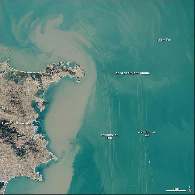
• The image of Figure 94 was released on Feb. 13, 2015 in ESA's 'Earth from Space video program.' Las Vegas with its grid-like urban plan is visible near the center. Sitting in a basin of the Mojave Desert, the city is surrounded by a number of mountain ranges. 92)
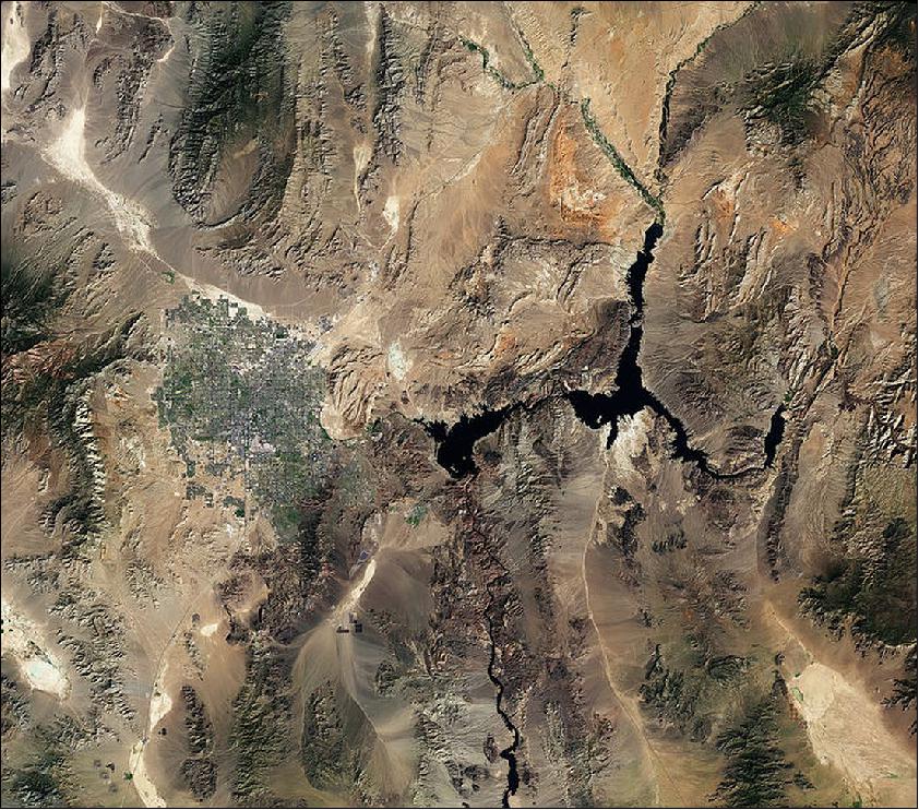
Legend to Figure 94: Zooming in southeast of the city one can see large, dark shapes in one of the desert valleys. These are solar panels of a large-scale plant called Nevada Solar One. The plant harnesses enough energy to power an estimated 14 000 homes a year. - Satellites can assist in the selection of sites of solar power plants by providing sunshine maps that combine information on overall solar irradiance and average cloudiness. Along with other space-derived products such as digital elevation models, this can help sustainable energy companies pinpoint areas best suited for exploiting solar energy.
The large dark area pictured is Lake Mead, the largest reservoir in the country. It primary source is the Colorado River, flowing in from the east and out to the south. This massive reservoir was established in the early 1930s by the construction of the Hoover Dam on the Colorado River. Drought and increased water demand in recent years have resulted in a decline in water levels, hitting record lows last summer. The lake and surrounding area form the Lake Mead National Recreation Area, where visitors can go boating, swimming, fishing, hiking, biking and camping.
• January 27, 2015: Authorities in the Indian states of Jammu and Kashmir are concerned that a landslide blocking the Tsarap River (also called the Phuktal River) may lead to a damaging flood downstream. 93)
- The landslide, which reportedly occurred on December 31, 2014, sent enough fine-grained debris into the river to create an earthen dam. As of January 20, 2015, that dam was about 600 m long, according to an analysis of satellite imagery collected by the ISRO's (Indian Space Research Organization) CartoSat-2. The artificial lake that formed behind the dam was nearly 8 km long and covered about 55 hectares (300 acres). Aerial surveys suggest the mound of debris blocking the river was about 60 m high.
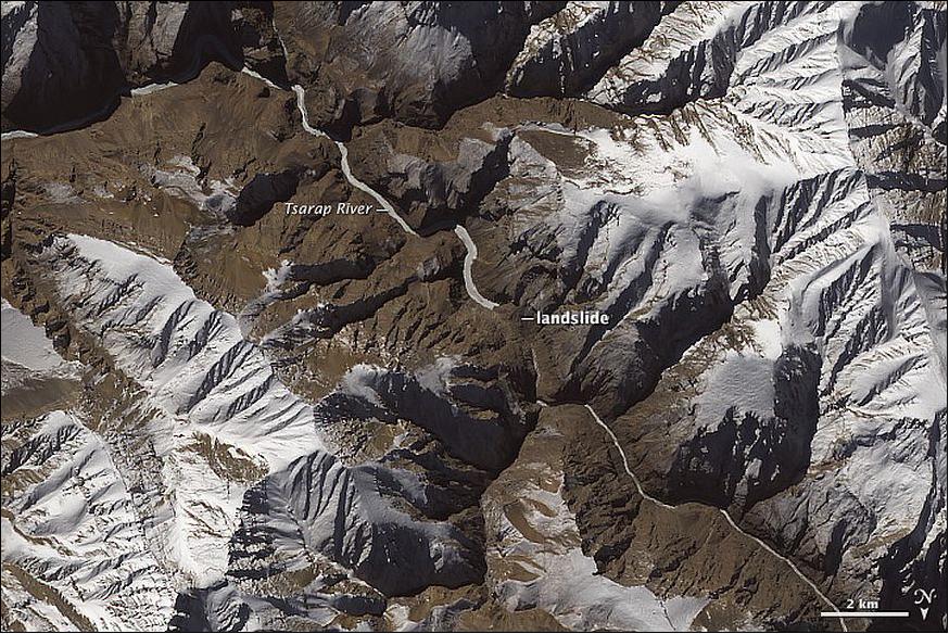
Legend to Figure 95: Notice that the river appears wider upstream of the landslide. The river also appears brighter after the landslide because the surface has frozen and a fresh coat of snow coats the ice. After surveying the situation on January 18, a team of civilian and military engineers recommended that people who live downstream move to higher ground. They also discouraged authorities from using explosives to clear the blockage as doing so could trigger additional landslides. While the chance of a catastrophic flood is lower with the lake frozen, the risk will increase when temperatures rise in the spring. As a precautionary measure, authorities have closed the Chadar ice trek, a popular route that involves hiking on frozen river ice downstream of the blockage.
• January 27, 2015: The Landsat-8 spacecraft is operating nominally and acquires OLI and TIRS data. However, the TIRS level-1 processing remains suspended. 94) 95)
- On December 19, 2014, the TIRS instrument on Landsat-8 was reconfigured due to detection of anomalous current levels associated with the scene select mirror encoder electronics. Since that time substantial testing has been conducted to isolate the root cause of the problem and to evaluate options for returning to routine operations. - During this time, TIRS data has been routinely collected with OLI data, but due to the lack of definitive calibration coefficients the processing of TIRS data to level-1 products has been suspended.
- Once a plan to return to normal operations has been defined, the backlog of TIRS data that have been collected will be processed to Level-1 products. Updates to the status of plans to resume normal operations will be provided periodically.
• The Landsat-8 image of Figure 96 was released on Jan. 30, 2015 showing Corsica, the most mountainous island of the Mediterranean Sea. About 40% of the island's surface area is dedicated to nature reserves, and its mountains are a popular destination for hiking. For beachgoers, the island boasts over 1000 km of coastline. 96)
- Near the northeastern coast, one can see the island's largest coastal lagoon, the Etang de Biguglia. This nature reserve has been noted for its support of numerous breeding and wintering waterbirds, as well as the vulnerable Hermann's tortoise and long-fingered bat.
- This lagoon is one of the over 2000 sites worldwide considered to be wetlands of international importance by the Ramsar Convention, an intergovernmental treaty for the sustainable use of wetlands. The World Wetlands Day is observed on 2 February, the anniversary of the signing of the Convention.
- ESA has been assisting the Ramsar Convention for a decade through the GlobWetland project, which provides satellite data to be used to monitor these precious resources. The next phase of the project, called GlobWetland Africa, will collaborate closely with ESA's TIGER initiative, which trains African water authorities and researchers in exploiting satellite data and Earth observation technology for sustainable water resource management.
- The Etang de Biguglia is not the island's only Ramsar site: further inland in the central-north part of the island is an active raised bog, home to a number of protected bat, reptile, bird and amphibian species.
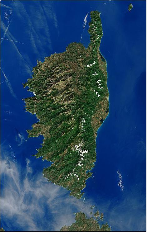
• The Landsat-8 image of Figure 97 was released by ESA on January 23, 2015 showing parts of the Swiss and Italian Alps as well as the Aletsch Glacier, the largest glacier in the Alps located in the center of the image. The glacier originates in a large, flat area of snow and ice high in the mountains called Concordia, where three smaller glaciers converge. It extends south, and its meltwater creates the Massa River in the valley below. Owing to climate change, the glaciers in this region are showing long-term retreat. The melting ice has given birth to new lakes, which pose risks such as flooding and landslides to communities at lower level. 97)
- Aletsch and the surrounding mountains are part of the Jungfrau-Aletsch protected area, a UNESCO World Heritage site. The area is of major importance to scientific research in geology, geomorphology, climatic change, biology and atmospheric physics. It features a wide diversity of ecosystems, and its landscape has played an important role in European art, literature, mountaineering and alpine tourism.
- One particularly popular tourist destination is the Swiss city of Interlaken, located between lakes Thun and Brienz, seen in the upper part of the image. From the city, locals and visitors alike have easy access to the mountains and water bodies, and can partake in a variety of outdoor activities during all seasons.
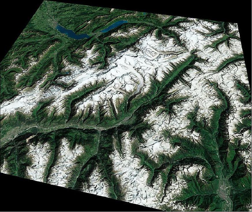
• 2014 update: Landsat imagery provides the United States and the world with continuous, consistent inventory and monitoring of critically important global resources. Supplying an unprecedented record of global land cover status and change for over 40 years, Landsat imagery is an essential "national asset" which has made and continues to make critical "contributions to U.S. economic, environmental, and national security interests." Because Landsat imagery is used most often by governmental and other non-commercial entities, the general lack of market forces makes estimating the economic value of Landsat data challenging. However, cost savings from operational efficiency improvements, avoided alternative replacement costs (assuming Landsat data were not available), and opportunity costs related to economic and environmental decision-support can be used to estimate the value of Landsat data. 98)
• Dec. 19, 2014: A small portion of underwater structures of the Great Bahama Bank is pictured in Figure 98. Sitting north of Cuba, the bank is made of limestone – mainly from the skeletal fragments of marine organisms – that has been accumulating for over 100 million years. Currents sculpted these underwater sediments into the wavy pattern we see along the bottom of the image, just a few meters deep. 99)
The shallow waters drop off into the deep, dark water of an area known as the Tongue of the Ocean. With depths of up to about 4000 m, this trench surrounded by islands, reefs and shoals has an opening to the Atlantic Ocean at its northern end. The trench was carved during the last Ice Age when the land was still above sea level and exposed to erosion from draining rainwater. As the Ice Age ended and the massive ice sheets across the globe melted, global sea levels rose and flooded the canyon.
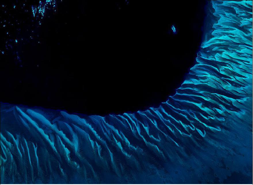
The MODIS image of the Great Bahama Bank of Figure 99 provides a much broader view of the area, including the Tongue of the Ocean. 100)
• Nov. 7, 2014: The Landsat-8 image of Figure 100 was released by ESA on Nov. 07, 2014. It shows part of the Middle East, with the Jordan Rift Valley running north to south. The most prominent feature in this image is the Dead Sea: the lowest point on Earth's surface, with 427 m below sea level. The Dead Sea is 50 km long, 15 km wide at its widest point, and 306 m deep. The extremely high salinity (34.2%) means fish cannot live in this water body, although there are bacteria and fungi. 101)
- With the Jordan River as its main source of water, the Dead Sea is an ‘endorheic' basin, meaning that the water has no outflow. Nonetheless, the water level has been dropping, an effect of the diversion of incoming water from the river.
- Note the greenish rectangles just south of the Sea. This is a large complex of mineral evaporation ponds used to produce sodium chloride and other salts for the chemical industry and human and animal consumption. These ponds are separated from the northern part of the Dead Sea by what once was the Lisan Peninsula but lowering water levels have exposed the sea bed, dividing the two sections completely.
- Throughout the rest of the image one can see built-up areas such as Amman, the capital of Jordan, in the upper right and Jerusalem near the green hills west of the Dead Sea. Further west we can see green patches of agriculture on the coastal plain, with Tel Aviv on the Mediterranean coast. - In the lower-left corner of the image, one can clearly see the division between Israel and the Gaza Strip not only by the outline of the border, but in the difference in agricultural practices.
• Oct. 26, 2014: On October 17, 2014, the eye of category 3 Hurricane Gonzalo passed right over Bermuda. The storm knocked out power to most of the island and caused between $200–$400 million in property damage, though it did not cause any deaths. The potent storm also stirred up the sediments in the shallow bays and lagoons around Bermuda, spreading a huge mass of sediment across the North Atlantic Ocean. 102)
OLI ( Operational Land Imager) on the Landsat 8 satellite acquired the two natural-color views of Bermuda in Figures 101 and 102. After the storm, visible plumes of sediment stretch 25 to 30 km from Bermuda. They extend mostly to the south and east of the island, suggesting that the last winds from the storm may have been out of the northwest. The suspended sediments were likely a combination of beach sand and carbonate sediments from around the shallows and reefs.
Coral reef and carbonate island environments—Bermuda is a classic example—produce large amounts of calcium carbonate (CaCO3) mainly in the form of aragonite and magnesian calcite. One island can produce as much CaCO3 as several hundred square kilometers of open ocean. But unlike the calcium carbonate produced in the open ocean by coccolithophores, foraminifera, and pteropods, the sediment produced by reefs stays on the reef flats (where there is coralline algae that also produces carbonate). It builds up over time and forms islands.
These stores of calcium carbonate sediments can get moved from the shallows to the deep ocean by storms or density flows. The strong winds of storms like Gonzalo can move a large amount of sediment off the shallow islands in a single event. Density flows can happen when the shallow water on the reef flat is cooled by a weather system, making it more dense than the surrounding ocean water, and it sinks to the deep ocean, taking sediments with it.
Storm-induced export of carbonate sediments into the deep ocean—where they mostly dissolve—is a significant process in the ocean's carbonate and carbon cycles. It's also important for the eventual neutralization of excess carbon dioxide entering the oceans because of increasing atmospheric CO2 concentrations from fossil fuel combustion. The dissolution of calcium carbonate is an important process in the carbon cycle; it is one of the ways that the oceans naturally balance the addition of carbon dioxide to ocean waters. However, as more CO2 is added to the surface waters due to rising atmospheric concentrations, it is becoming increasingly difficult for coral and coralline algae to make calcium carbonate.

• Sept. 29, 2014: The greens and blues of the ocean color from NASA satellite data (Figure 103) have provided new insights into how climate and ecosystem processes affect the growth cycles of phytoplankton—microscopic aquatic plants important for fish populations and Earth's carbon cycle. 103)
Climate change will unquestionably influence global ocean plankton because it directly impacts both the availability of growth-limiting resources and the ecological processes governing biomass distributions and annual cycles. Forecasting this change demands recognition of the vital, yet counterintuitive, attributes of the plankton world. The biomass of photosynthetic phytoplankton, for example, is not proportional to their division rate. Perhaps more surprising, physical processes (such as deep vertical mixing) can actually trigger an accumulation in phytoplankton while simultaneously decreasing their division rates. These behaviors emerge because changes in phytoplankton division rates are paralleled by proportional changes in grazing, viral attack and other loss rates. Here, the trophic dance between predators and prey is discussed, how it dictates when phytoplankton biomass remains constant or achieves massive blooms, and how it can determine even the sign of change in ocean ecosystems under a warming climate. 104)
At the bottom of the ocean's food chain, phytoplankton account for roughly half of the net photosynthesis on Earth. Their photosynthesis consumes carbon dioxide and plays a key role in transferring carbon from the atmosphere to the ocean. Unlike the plant ecosystems on land, the amount of phytoplankton in the ocean is always followed closely by the abundance of organisms that eat phytoplankton, creating a perpetual dance between predators and prey. This new analysis shows how tiny imbalances in this predator-prey relationship, caused by environmental variability, give rise to massive phytoplankton blooms, having huge impacts on ocean productivity, fisheries and carbon cycling.
The continuous year-in and year-out measurements provided by NASA's ocean color satellites have dramatically changed our understanding of phytoplankton dynamics on the Earth.
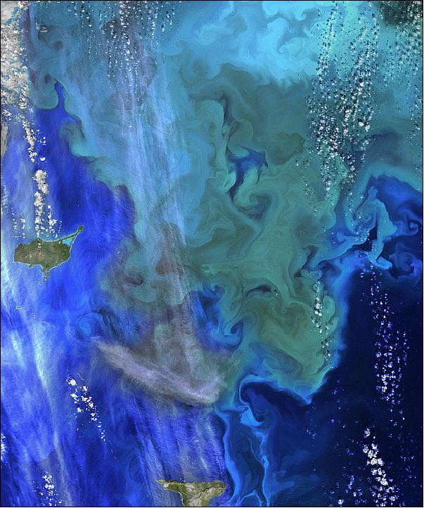
In early September 2014, the SLI (Sustainable Land Imaging) Office at NASA/GSFC announced, that the following companies have been awarded contracts to carry out the SLI 'Reduced Instrument Envelope Study'. • BATC (Ball Aerospace & Technologies Corporation) of Boulder, CO • Exelis Inc., Geospatial Systems of Fort Wayne, IN • Lockheed Martin Space Systems Company of Greenbelt, MD • Northrop Grumman Systems Corporation, Aerospace Systems of Redondo Beach, CA • Raytheon Company of El Segundo, CA • SST-US (Surrey Satellite Technology US LLC) of Englewood, CO. The study focuses on investigating mid-term capabilities and technologies for instruments that may enable more efficient implementation of the SLI program objectives to continue the Landsat heritage of measurements. The study contract awards are intended to enable contractors to perform a more detailed analysis of techniques and trends that lead to reduction in size and mass of spaceborne Earth-imaging instruments, potentially resulting in cost savings to the U.S. Government while still meeting the SLI program objectives. These studies will be of 6-month duration. Landsat data provide a consistent and reliable foundation for research on land use change, forest health, and carbon inventories, and changes to our environment, climate, and natural resources. Additionally, the free and open availability of the Landsat data enables the measurements to be used routinely by decision makers both inside and outside the Government, for a wide range of natural resource issues, including water resource management, wildfire response, agricultural productivity, rangeland management, and the effects of climate change. The U.S. Government has committed to continue the Landsat program and its invaluable data stream. To continue data collection beyond Landsat-8, the Administration proposes to design and implement a spaceborne system to provide global, continuous Landsat-quality multispectral and thermal infrared measurements for at least the next 25 years. The satellite system may be combined with alternative sources for Landsat-quality data, either procured through commercial approaches or through partnership agreements, as they become available. In accordance with Administration objectives, NASA will lead the system design study in close collaboration with the USGS (United States Geological Survey) and be informed by existing knowledge of current and desired capabilities. The aim of the study will be to define a programmatically sustainable system that balances measurement capability, likelihood of data continuity (minimizing risks of gaps to the extent possible), and cost/affordability over the lifetime of the program. Technology infusion over the lifetime of the program will be considered as a feature of the long-term sustainable program. In FY 2014, NASA will initiate the definition of a sustained, spaceborne, global land imaging capability for the nation, ensuring continuity following LDCM. Near-term activities led by NASA, in cooperation with USGS, will focus on studies to define the scope, measurement approaches, cost, and risk of a viable long-term land imaging system that will achieve national objectives. Evaluations and design activities will include consideration of stand-alone new instruments and satellites, as well as potential international partnerships. It is expected that NASA will support the overall system design, flight system implementation, and launch of future missions, while USGS will continue to fund ground system development, post-launch operations, and data processing, archiving, and distribution. |
• August 27, 2014: Ethiopia's Danakil Depression (or Afar Depression) exhibits some uncommon wonders: lava that burns blue, bright yellow hot springs, and lakes of bubbling mud. These otherworldly oddities are all manifestations of a tectonic process called continental rifting. In other words, the Earth is pulling apart at the seams here. 106)
In northeastern Africa, the Arabian, Somali, and Nubian (or African) plates are separating, thinning Earth's crust as they pull apart. The Danakil Depression lies between the Danakil Alps (east) and the Ethiopian Plateau (west), which were once joined until the rifting process tore them apart. The land surface is slowly sinking, and Danakil Depression will someday fill with water as a new ocean or great lake is born. But for now, the region is full of other interesting liquids.
The image (Figure 104) shows a few of the diverse and compelling features of the Danakil Depression. Chief among them is Gada Ale, the northernmost volcano in the Erta Ale volcanic range. Gada Ale is a 287 m stratovolcano built of lava and ash, and it has a crater lake full of boiling mud and sulfurous gases. Basalt lava from the volcano paints the surrounding terrain a dark hue, with the youngest flows being the darkest colors in the satellite image.
Just southwest of Gada Ale, a 2 km wide salt dome has pushed ancient lava flows up to heights of 100 m. North of Gada Ale, a salt lake (Lake Karum) lies 116 m below sea level. To the south lies the Catherine Volcano, a 120 m circular shield surrounded by a tuff ring (an amalgamation of volcanic ash). With gently sloping sides of basaltic lava, the volcano has been dated at less than one million years old. In the center of that tuff ring is a small, salty lake fed by thermal springs.
The Afar people have survived in this unforgiving region for at least 2,000 years, mining and selling the plain's abundant salt, which was once used as currency in Ethiopia. The harsh desert also has created an ideal exposure for the tectonic rifting—a process that often occurs on the recesses of the ocean seafloor or elsewhere on land where younger sedimentary rocks obscure the geologic record.
• August 20, 2014: Retreat of the Yakutat Glacier in Alaska. Natural processes and human-caused warming have combined to bring rapid change to a glacier in southeastern Alaska. The Yakutat Glacier is one of the fastest retreating glaciers in the world. It is the primary outlet for the 810 km2 Yakutat ice field, which drains into Harlequin Lake and, ultimately, the Gulf of Alaska. 107)
Legend to Figures 105 and 106: Landsat satellites captured this pair of images showing changes in the glacier and lake. The TM (Thematic Mapper) on Landsat -5 acquired the image of Figure 106 on August 22, 1987; the OLI (Operational Land Imager) on Landsat-8 captured the image of Figure 105 on August 13, 2013. Snow and ice appear white and forests are green. The brown streaks on the glaciers are lateral and medial moraines.
Over the past 26 years, the glacier's terminus has retreated more than 5 km. What is causing the rapid retreat? University of Alaska glaciologist Martin Truffer and colleagues pointed to a number of factors in their 2013 study published in the Journal of Glaciology. The chief cause is the long-term contraction of the Yakutat Ice Field, which has been shrinking since the height of the Little Ice Age. - Once part of a much larger ice field, Yakutat has been contracting for hundreds of years. As other nearby glaciers retreated, Yakutat ice field was cut off from higher-elevation areas that once supplied a steady flow of ice from the north. With that flow cut off, there simply is not enough snow falling over the low-elevation Yakutat ice field to prevent it from retreating.
Beyond this natural change, human-caused global warming has hastened the speed of the retreat. Between 1948–2000, mean annual temperatures in Yakutat increased by 1.38°Celsius . Between 2000 and 2010, they rose by another 0.48°C . The warmer temperatures encourage melting and sublimation at all ice surfaces exposed to the air.
In the past few years, the breakdown of a long, floating ice tongue has triggered especially dramatic changes in the terminus of the Yakutat glacier. For many years, Yakutat's two main tributaries merged and formed a 5 km calving face that extended far into Harlequin Lake. In the past decade, satellites observed a rapid terminus retreat and the breakup of the ice tongue in 2010. As a result, the calving front divided into two sections, with one running east-west and another running north-south.
• July 2, 2014: The Landsat 8 satellite is helping researchers to spot organisms like aquatic algae from space, gathering information that could direct beachgoers away from contaminated bays and beaches. With improved sensors and technology on the latest Landsat satellite, researchers can now distinguish slight variations in the color of coastal water due to algae or sediments to identify potential problem areas. 108)
- The OLI (Operational Land Imager) on Landsat-8 added the "New Deep Blue" band (433-453 nm) to pick up dark blue colors to help studies that are looking at coastal areas, both of lakes and oceans. Pollutants from land impact fresh and salt-water ecosystems including coral reefs.
Beyond the blue of the water, a study of John Schott of RIT (Rochester Institute of Technology) at the University of Rochester, N. Y. is paying attention to three colors to decipher what's in Lake Ontario: green, yellow and grey. Green indicates the presence of chlorophyll, the molecule found not only in land plants but in lake algae. The yellow color is decaying plant matter. The gray color, apparent from a combination of Landsat's bands, comes from particulates like dust and soil, or from dead algae that have lost their chlorophyll.
- After paddling out in boats and testing the waters on the same day Landsat 8 passed overhead, the team compared the water samples to the satellite data. The comparisons are used to create tables and computer programs that can use the satellite data to help determine water quality and composition. This summer, the team plans to sample the harmful algal blooms that start small in Lake Ontario's bays and rivers – which could grow and cause water quality and public health concerns.
- It's not just the algae floating on the surface that Landsat-8 can spy. Scientists with the Michigan Tech Research Institute are tracking the spread of Chladophora, a hair-fine algae that attaches to shallow water rocks, or the shells of dead invasive zebra and quagga mussels. Occasionally, due to storms in the Great Lakes, the algae slough off the rocks, and cover the beach in a green decaying mess.
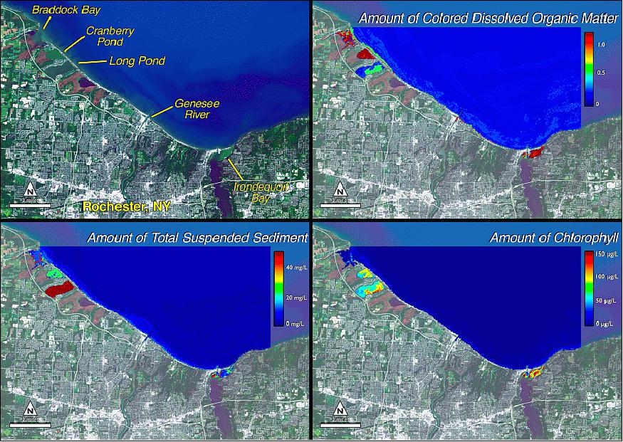
- Sediment swirls and chlorophyll whirls: Researchers in Belgium are looking at the swirls of sediments created by wind turbines in near shore waters. Wind companies are required to monitor the environmental impact of the turbines, explained Quinten Vanhellemont, a scientist with the Royal Belgian Institute for Natural Sciences, and Landsat-8 has the spatial resolution – and the sensitivity – to pick up some of the smaller features. The resolution and sensitivity of the imager on board makes it an ideal sensor for coastal water applications.
- At NASA/GSFC, scientists in the Ocean Ecology Laboratory are looking to Landsat-8 as well. They have created open-source software that researchers use to analyze satellite data for studies on marine phytoplankton chlorophyll concentration other water constituents. Currently they use satellites that take the big view, but Bryan Franz, a research oceanographer at Goddard, worked with Vanhellemont to see how well Landsat 8 data could be processed to determine chlorophyll patterns in coastal waters. It shows promise, Franz said. He plans to add Landsat 8 data to the software this summer to see how the ocean research community will use it (Ref. 108).
• The image of Figure 109 was released on July 1, 2014 in NASA's Earth Observatory program. Turkmenistan is a desert country that lies east of the Caspian Sea and borders Iran, Afghanistan, Uzbekistan, and Kazakhstan. Annual precipitation across the country ranges from 300 mm in the mountains to 80 mm in the desert northwest. In a country just larger than California, nearly 80% of the land is defined as desert. 109)
Despite the harsh, dry environment, these desert expanses were once part of the ancient east-west trade route between the Roman Republic and Han Dynasty. As part of the Silk Road from Europe to China, Turkmenistan was coveted by the Mongols, Turks, and Russians. Each have taken turns ruling the region over the past two millennia.
In the 18th century, people in the region started to think about taming the great Garagum Desert (also known as the Kara Kum or Karakumsky). The idea was to bring water southward from the Amu-Darya River, which runs through the northern desert. Under Soviet rule in the 1950s, the idea was realized. - In a feat of engineering, water from the Amu-Darya was channeled more than 1,300 km to irrigate the southern lands. Under construction from 1954 to 1988, the Garagum Canal project opened a million hectares of land to farming of cotton, wheat, melons, and animal fodder. Today, agriculture accounts for 7% of Turkmenistan's gross domestic product and employs nearly half of the country's workforce.
In this natural-color Landsat-8 image acquired on April 18, 2014, the Hanhowuz (Khauzkhan) Reservoir jumps out as a splash of turquoise amidst desert browns. The reservoir was constructed in a natural depression to capture winter runoff and overflow from the canal for use later during the driest periods of summer. Phytoplankton thrive in the warm waters, as do many commercial fish—including Aral barbel, asp, and catfish.
In the image of Figure 109, Garagum Canal is the brown ribbon dropping down from the upper right corner and heading south and east from the reservoir. A portion of the canal is diverted, and one can see the brown sediment-laden water entering the reservoir from the east and dropping its load of suspended sediments. The water that leaves is turquoise and travels west to irrigate the Tedjen Oasis. Roughly rectilinear farmlands appear on either side of that section of the canal.
Water is vital to the existence of Turkmenistan, but the canal that started as an engineering wonder for arid lands has also turned out to be an environmental tragedy. The canal has starved the Aral Sea, which has lost about 90% of its water since the canal's creation. Making matters worse, inefficient earthen canals lose nearly half of the canal water between the Aral Sea and Turkmenistan's farms. Smudges of green-grey along their sides of the canal (north of the reservoir) show where water has seeped out.
• The image of Figure 110 was released on June 18, 2014 in NASA's Earth Observatory program. The double oxbow — called the loop — is known as an "entrenched meander" by geologists, the Loop's canyon walls are about 150 m high. The lower canyon walls are part of the Hermosa Formation, a group of sedimentary rock layers that formed about 300 million years ago. At the narrowest point, just 150 m of rock separate the channels of the East Loop; the slightly wider neck of the West Loop measures about 520 m. As the Colorado River continues to erode the canyon wall, it will eventually punch through and create a new channel, leaving an oxbow lake and later a rincon. 110)
How the entrenched meanders of the Colorado River (and other rivers that flow through the Colorado Plateau) formed has intrigued western geologists since a team of explorers led by John Wesley Powell passed through the Canyonlands region in 1869. Were meanders established by ancestral rivers that flowed on softer sediments long before tectonic forces uplifted the Colorado Plateau? Or was it something about the rock of the Colorado Plateau that determined the shape and distribution of oxbows and meanders?
• Figure 111 is a Landsat-8 image of the southwestern coast of Greenland, released by ESA on June 13, 2014. Multiple ice streams, that drain the Greenland ice sheet, are pictured in this satellite image. 111)
- Covering more than 2,000,000 km2, Greenland is the world's largest island and home to the second largest ice sheet after Antarctica. Scientists, using data from Earth-observing satellites, have discovered that the rate of ice sheet melting is increasing. Between 1992 and 2012, Greenland was responsible for adding about 7 mm to the average global sea level. Many areas in Greenland – especially along the coast – are losing up to 1 m of ice thickness per year.
- Melting ice sheets, caused by rising temperatures and the subsequent rising of sea levels, is a devastating consequence of climate change, especially for low-lying coastal areas. In addition, the increased influx of freshwater into oceans affects the salinity, which in turn impacts global ocean currents – a major player in the regulation of our climate.
- Monitoring the effects of climate change on the cryosphere and oceans using Earth-observing satellites is the main topic of an event which took place on June 13, 2014 at the Royal Society in London. The event was jointly organized by ESA and the UK Space Agency (UKSA) with the aim to provide an overview of the outcome and scientific significance of the achievements of the Climate Change Initiative with a focus on new climate data sets from space, the cryosphere and the ocean.
Legend to Figure 111: In the lower part of the image, one can see icebergs speckling the waters of a fjord, with the mountainous Nuussuaq Peninsula visible along the bottom of the image.
• June 2014: During the early on-orbit period of Landsat-8, ground-based measurements indicated a significant error in the radiance produced from TIRS (Thermal Infrared Sensor), especially in Band 11. 112)
After several months of analysis, the NASA TIRS team suspected a stray light issue with the sensor. Scans of the moon by the TIRS instrument have confirmed this. Users were notified of the issue through the Landsat-8 Calibration Notices (https://web.archive.org/web/20161129095927/https://landsat.usgs.gov/calibration_notices.php) and the USGS Landsat Updates (http://landsat.usgs.gov/about_Landsat_Updates.php), starting in August 2013.
- During the early on-orbit period of Landsat-8, ground-based measurements indicated a significant error in the radiance produced from the TIRS. After collecting additional ground measurements through the summer of 2013, this error was estimated to be 0.29 W/m2/sr/mm for Band 10 and 0.51 W/m2/sr/mm for Band 11.
- All errors showed that TIRS reported a higher radiance than the ground measurements, as shown in the left graph of Figure 112. The right graph shows the results after accounting for this average radiance error, which is the calibration adjustment that was implemented for reprocessing in February 2014. The adjustment accounts for the apparent bias, but there remains a significant amount of variance, especially within Band 11.
• May 22, 2014: After 14 years of drought, Lake Powell (on the Colorado River) was at 42 % of its capacity as of May 20, 2014. The low water levels are evident in these images of Figures 113 and 114, which were acquired by the Landsat-8 satellite on May 13, 2014. White bleached rock show where Lake Powell's shore is when the reservoir is at capacity. In Figure 113, which shows the northern section of Lake Powell, a muddy Colorado River flows through a largely empty lakebed. The Figure 114 shows a section of the reservoir closer to the Glen Canyon Dam and popular with boaters. Here, Halls Creek Bay is clearly smaller than it is in the National Park Service map of Lake Powell. 113)
Legend to Figures 113 and 114: Water rules the western United States. Not only does it sustain cities, but it also fuels the economy. It's both a primary source of electricity and the foundation for agriculture. For all that, water is often not available in the Southwest and Intermountain West. To ensure a steady supply, the United States built a series of reservoirs throughout the 20th century. The two largest, Lake Mead and Lake Powell, sit behind massive dams on the Colorado River and provide water and electricity to several western states.
It is normal for water levels to fluctuate in the reservoir depending on how much water flows in from snow and rain and how much flows out to meet needs. However, it has been dry in all but three of the past 14 years. At the beginning of 2000, Lake Powell was at 94% of capacity. By October 2013 (the beginning of the 2014 water year), water levels had dropped to a low of 50% capacity, according to the Bureau of Reclamation, the agency that manages the reservoir. The Earth Observatory's World of Change shows this annual fluctuation and overall decline. With slightly above average snowpack in the basin that feeds the lake, water levels are expected to rebound to about 51% of capacity by October 2014, the end of the current water year.
While the drop in water levels are worrying for those who generate electricity or use the water for agriculture, the lower water levels may be a draw for recreation. Boaters coming to Lake Powell in the spring of 2014 will find beaches and rock formations that are usually underwater. Bullfrog Bay is the starting point for many boat rentals. The popularity of the spot is evident in the lower image: boats dot the surface of the water, just tiny white flecks at this scale.
• April 25, 2014: Of the roughly 1,550 volcanoes that have erupted in the recent geologic past, 113 are found on Kamchatka. Forty Kamchatkan volcanoes are "active," either erupting now or capable of erupting on short notice. The Operational Land Imager (OLI) on Landsat-8 captured activity at five of them during a single satellite pass on April 14, 2014. The imagery can be found at the following reference. 114)
• On April 8, 2014, the NASA Earth Observatory series released an image of Landsat-8 which spotted a perfect alluvial fan in Kazakhstan's Almaty province on September 9, 2013 (Figure 115). 115)
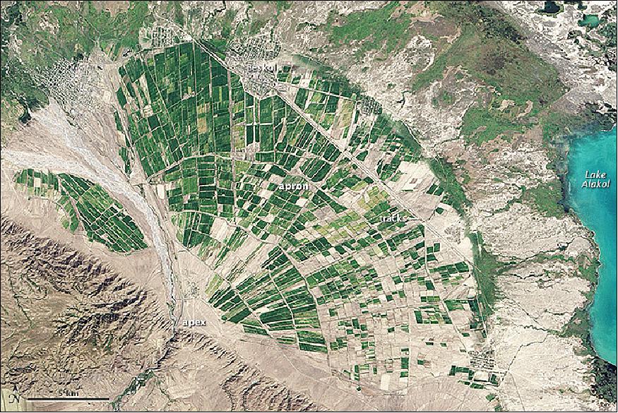
Legend to Figure 115: In the lower left of the image, the Tente River flows through a narrow channel in the foothills of the Dzungarian Alatau range. Where the Tente emerges from the hills near Lake Alakol, it spreads out and becomes a braided stream. The movement of the channel over time has left a large fan that's about 20 km across at its widest point.
Mountain streams are usually confined to narrow channels and tend to transport sizable amounts of gravel, sand, clay, and silt—material that geologists call alluvium. The type and quantity of alluvium transported depends on the volume of the water flow and the gradient of the stream. Larger rivers pick up more alluvium than smaller ones; fast-flowing streams on steep slopes transport coarser sediment than slow-moving ones on shallow slopes.
The narrowest point of an alluvial fan—closest to the mountain front—is known as the apex; the broader part is called the apron. Alluvium deposited closer to the apex tends to be coarser than the material that makes up the apron. Alluvial fans are more likely to form in deserts because there is plenty of loose alluvium and not much vegetation to prevent stream channels from shifting.
Alluvial fans in arid areas are often used for agriculture because they are relatively flat and provide groundwater for irrigation. This fan is no exception. The blocky green pattern across the apron are fields or pasture land. A number of towns and villages, including Usharal and Beskol, are visible along the fan's outer edge. The straight feature cutting through Beskol and along the northeastern portion of the fan are railroad tracks.
• In March 2014, the Landsat-8 spacecraft and its payload are operating nominally. 116)
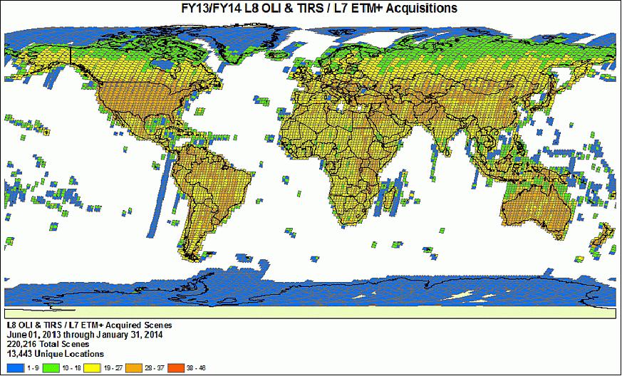
• Feb. 25, 2014: Large landslide detected in Southeastern Alaska. Using imagery from the Landsat-8 satellite, scientists have confirmed that a large landslide occurred in southeastern Alaska on February 16, 2014. A preliminary estimate suggests the landslide on the flanks of Mount La Perouse involved 68 million metric tons of material, which potentially makes it the largest known natural landslide on Earth since 2010.
Legend to Figure 118: The avalanche debris appears light brown compared to the snow-covered surroundings. The sediment slid in a southeasterly direction, stretching across 7.4 km and mixing with ice and snow in the process. The slide was triggered by the collapse of a near-vertical mountain face at an elevation of 2,800 m, according to Colin Stark, a geophysicist at the Lamont-Doherty Earth Observatory at Columbia University.
Stark first became aware that a landslide may have occurred when a rapid detection tool that sifts through data collected by a global earthquake monitoring network picked up a signal indicative of a fairly significant event. The earthquake sensors detect seismic waves—vibrations that radiate through Earth's crust because of sudden movements of rock, ice, magma, or debris.
While both earthquakes and landslides produce both high-frequency and low-frequency waves, landslides produce more low-frequency waves on balance than earthquakes. Most earthquake detection tools are focused on high-frequency waves, but the detection tool Stark was using the Global CMT (Centroid-Moment-Tensor) Project, also looks closely at low-frequency waves, meaning it is more likely to detect landslides than other tools.
• Feb. 11, 2014: One year ago, on Feb. 11, 2013, NASA launched the Landsat-8 Earth-observing satellite from Vandenberg Air Force Base in California. The launch went perfectly, and 100 days later NASA transferred operational control to the USGS (U.S. Geological Survey). Landsat-8 then joined its predecessor satellites to provide a continuous record of change across Earth's land surfaces since 1972. 119)
- Landsat-8 is acquiring around 550 images/day – significantly more than the 400-image/day design requirement. Between Landsat-7 (launched in 1999 and still active) and Landsat-8, nearly 1,000 images/day are being collected. This is almost double the imagery collected three years ago, when Landsat-5 and -7 were operating together. The ability of Landsat-8 to image more frequently in persistently cloudy areas (e.g., humid tropics, high latitudes) is improving data collection in areas of critical importance for climate studies.
- Landsat-8's robust data processing system also enables images to be available for public use within five hours of their arrival at the USGS EROS (Earth Resources Observation and Science) Center in Sioux Falls, S.D. Since 2008, all Landsat data is free to all. Enhanced Landsat-8 data have quickly found their way into a wide range of operational applications, including forest health monitoring by the U.S. Forest Service, burn severity mapping by the USGS, NASA and the National Park Service, and cropland mapping by the National Agricultural Statistical Service.
- During the past 12 months, the USGS-EROS Center and NASA/GSFC have worked in close collaboration — putting the new satellite through its paces by steering it into its orbit, calibrating its detectors, collecting test images and certifying the mission for sustained operation.
- As partners in the Landsat program since its inception in the 1960s, USGS and NASA have distinct roles. NASA develops remote-sensing instruments and spacecraft, launches the Landsat satellites and validates their performance. The USGS then assumes ownership and operation of the Landsat satellites, in addition to managing ground-data reception, archiving, product generation and distribution.
• January 2014: The Landsat-8 spacecraft and its payload are operating nominally in 2014 with performance exceeding specifications in many respects. 120)
• January 10, 2014: Figure 119 is an OLI image of Guinea-Bissau and the Bissagos islands. Mangrove swamps are abundant along this coastline, acting as important feeding grounds for fish, birds and animals. Flowing from the east, the Geba River empties into the Atlantic Ocean, with the country's capital city of Bissau located on the river estuary. The city appears as a light brown area in the upper-central portion of the image. 121)
- Off the coast in the lower-left section of the image are the Bissagos (or Bijagós) islands – an archipelago of over 80 islands and islets. In 1996 the archipelago was declared a UNESCO Biosphere Reserve. A diversity of mammals, reptiles, birds and fish can be found on the islands, including protected or rare species such as the Nile crocodile, hippopotamus, African manatee and the common bottlenose dolphin. The archipelago has also been recognized as an important site for green sea turtles to lay their eggs.
- In the lower left corner, the island of Orango looks like a tree, with the waterways like branches and land appears as foliage. This island is the center of a national park, and is known for its matrimonial tradition where marriage is formally proposed by the women – who are also responsible for building the homes.
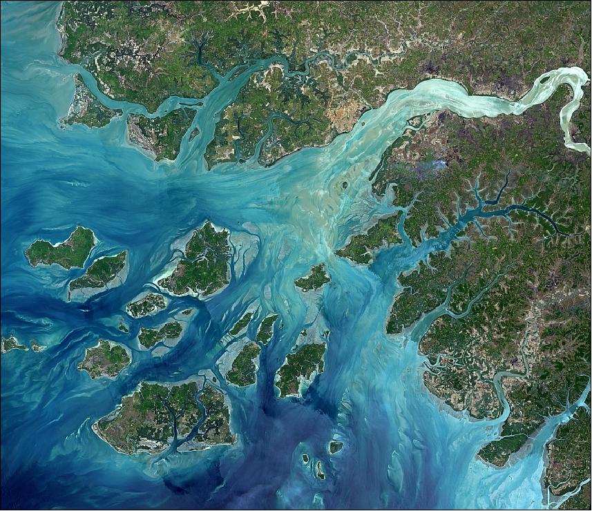
• Dec. 09. 2013: The coldest spot on Earth was found to be in Antarctica on the East Antarctic Plateau where temperatures in several hollows can dip below minus 92ºC on a clear winter night. Scientists made the discovery while analyzing the most detailed global surface temperature maps to date, developed with data from remote sensing satellites including the new Landsat 8, a joint project of NASA and the U.S. Geological Survey (USGS). 122)
The researchers analyzed 32 years' worth of data from several satellite instruments. They found temperatures plummeted to record lows dozens of times in clusters of pockets near a high ridge between Dome Argus and Dome Fuji, two summits on the ice sheet known as the East Antarctic Plateau. The new record of minus 93.2º C was set Aug. 10, 2010.
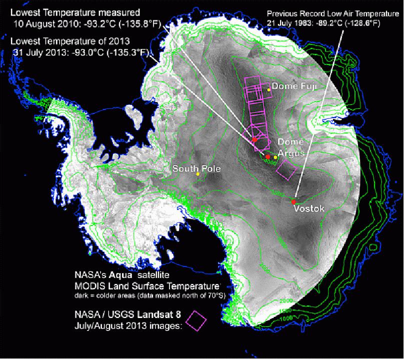
• Nov. 2013: The OLI instrument of Landsat-8 acquired imagery of lava flows in northern Chile, highlighting some of the distinctive features of a coulée. Lava domes tend to have steep, cliff-like fronts at their leading edge and wrinkle-like pressure ridges on their surfaces. The Chao is a type of lava dome known as a coulée. These elongated flow structures form when highly viscous lavas flow onto steep surfaces. 123)
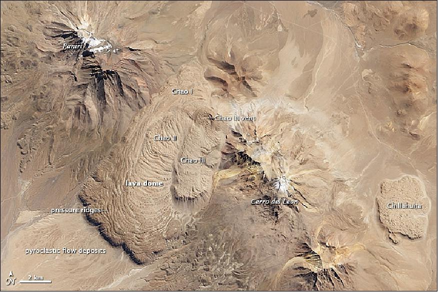
Legend to Figure 121: The Chao dacite sits between two volcanoes in northern Chile: the older and partially-eroded Cerro del Leon and the younger Paniri. The dome itself is a giant tongue of rock that extends southwest from the vent. Curved pressure ridges known as ogives dominate the surface of the 14 km dome.
Volcanologists estimate the Chao dacite dome formed over a period of about 100 to 150 years. A pyroclastic flow during the Chao I phase left light-brown deposits of tephra and pumice at the leading edge of the flow. Pyroclastic flows are avalanche-like events that bring mixtures of hot gas and semi-sold rocks surging down the flanks of volcanoes at speeds as fast as 100 km/hour.
This period was followed by the Chao II phase, when 22.5 km3 of lava erupted. This flow has 400 m tall fronts that stand out with their dark shadows on the southwest end. The final, Chao III phase added another 3.5 km3 of denser lava with a lower viscosity. This type of lava is less likely to form pressure ridges, so surfaces in this part of the flow are comparatively smooth.
• Oct. 22, 2013: Since its launch in February 2013, Landsat-8 has collected about 400 scenes of the Earth's surface/day. Each of these scenes covers an area of about 185 km x 185 km or 34,200 km2 for a total of 13,690,000 km2/day. An area about 40% larger than the United States, every day.
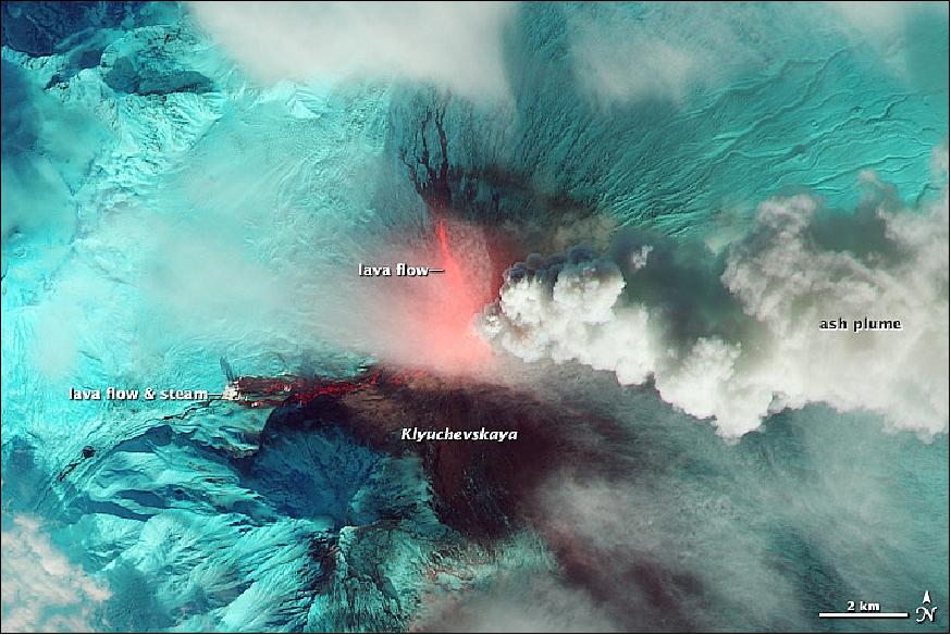
Legend to Figure 122: Located on Russia's Kamchatka Peninsula, Klyuchevskaya (also spelled Kliuchevskoi) is one of the world's most active volcanoes. More than 100 flank eruptions have occurred at the stratovolcano in the past 3,000 years, according to Smithsonian's Global Volcanism Program. Twelve confirmed eruptions have occurred since 2000.
Klyuchevskaya has been erupting since August 15, 2013, though the intensity of activity surged in October. The Kamchatka Volcanic Eruption Response Team (KVERT) reported a thick plume of ash and steam streaming from the summit on October 11. Subsequent days brought explosive eruptions, lava fountains, and volcanic tremors. At times, the ash plume rose from the summit (elevation 5 km) up to 7.5 to 10 km.
When OLI of Landsat-8 flew over in the afternoon on October 20, multiple lava flows streamed down Klyuchevskaya northern and western flanks. The false-color image of Figure 122 shows heat from the flows in SWIR, and green light. Ash, water clouds, and steam appear gray, while snow and ice are bright blue-green. Bare rock and fresh volcanic deposits are nearly black. 124)
• August 25, 2013: A study of Garden and Hog Islands of Lake Michigan observed by Landsat-8. 125)
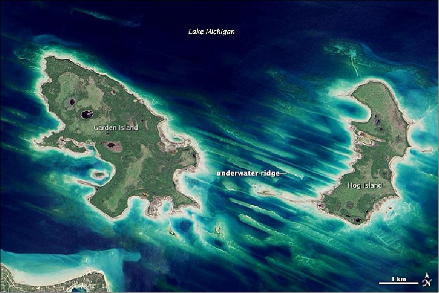
Legend to Figures 123 and 124: Over thousands of years, retreating glaciers scoured and carved out much of the basin that now holds Lake Michigan. But in some parts of the lake, patches of erosion-resistant rock still protrude above the water. A cluster of small islands in the far northern reaches of the lake—the Beaver Island archipelago—are composed of limestone bedrock covered with a layer of sand and gravel (glacial "till").
Except for Beaver Island, the largest of the group, the islands are unpopulated. About 700 people live on Beaver Island, mainly in a small town on the northern part of the island. A Native American community survived on Garden Island until as recently as the 1900s, but the size of the community dwindled until the last remaining resident died in the 1940s.
The OLI (Operational Land Imager) on Landsat 8 captured the top image (Figure 123) of Garden and Hog islands on May 24, 2013. The lower image, a broader view (Figure 124), shows Beaver Island and the other islands in the context of the great lake. Dense forests, swamps, and sandy beaches dominate the landscape. Offshore, deeper waters appear dark blue, while shallow areas are turquoise.
The shallows around Garden and Hog islands contain numerous parallel rock ridges interspersed by deeper channels. These reef areas offer ideal spawning ground for various species of fish, notably lake trout and perch. Federal and state resource managers have attempted to replenish depleted lake trout populations by stocking northern Lake Michigan waters.
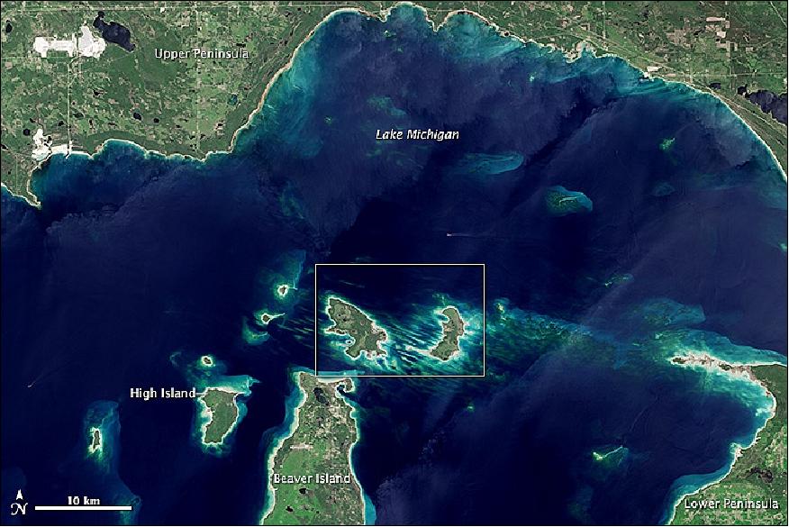
• On August 18, 2013, Mount Sakurajima (Japan) on the island of Kyushu erupted. The eruption lasted for about 50 minutes, sending ash and smoke across the bay into the city of Kagoshima, which is near the southwestern tip of the island of Kyushu in Japan. 126)
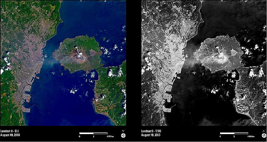
Legend to Figure 125: The color image (left) uses Landsat bands 4, 3 and 1 of OLI (Operational Land Imager). The black and white image (right) was acquired with TIRS (Thermal Infrared Sensor) in band 10 and displays the temperature differences. Warmer surfaces appear light gray to white in the thermal image, while cooler areas appear dark gray to black. While there are few clouds near the caldera, the bright land surface indicates the heat on the land near the volcano.
• In June 2013, the Silver Fire of 55850 hectar in size in New Mexico, USA, was observed by Landsat-8 repeatedly to give forest restoration specialists a means to analyze and determine where the burn destroyed vegetation and exposed soil – and where to focus emergency restoration efforts. 127)
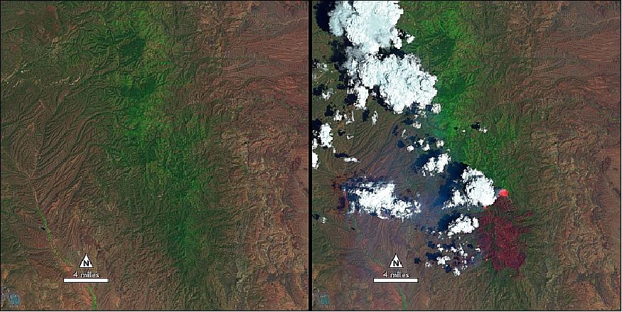
Legend to Figure 126: The red color in the right-hand picture means high-severity fire, and the red areas were concentrated in a watershed drainage that fed communities west of Las Cruces, N.M. The BEAR (Burned Area Emergency Response) teams are designed to go in as soon as the flames die down to help protect reservoirs, watersheds and infrastructure from post-fire floods and erosion.
Legend to Figure 127: As a wildfire starts to die down, fire managers can contact the Forest Service's Remote Sensing Applications Center in Salt Lake City to request maps that identify the high, moderate and low severity burns. When that call comes in, remote sensing specialist Carl Albury finds satellite imagery of the burned forest both pre- and post-fire.
In Landsat-8 imagery, two of the 11 spectral bands – the near-infrared band (No 5) and a short-wave infrared band (No 6) are used for hot spots. The near infrared reflects well from healthy vegetation, and the short-wave infrared bands reflect well from exposed ground. By comparing the normalized ratio of the near- and shortwave-infrared bands in the pre-fire image to the post-fire image, the burn severity can be estimated (Ref. 127).
1) "Pine Island Iceberg Under the Midnight Sun," NASA Earth Observatory, 26 Dec. 2017, URL: https://earthobservatory.nasa.gov/IOTD/view.php?id=91470
2) "Cape Horn: A Mariner's Nightmare," NASA Earth Observatory, 24 Dec. 2017, URL: https://earthobservatory.nasa.gov/IOTD/view.php?id=91472
3) "The Land Between the Lakes," NASA Earth Observatory, 15 Dec. 2017, URL: https://earthobservatory.nasa.gov/IOTD/view.php?id=91391&src=iotdrss
4) "A Growing City and a Deadly Landslide," NASA Earth Observatory, Dec. 5, 2017, URL: https://earthobservatory.nasa.gov/IOTD/view.php?id=91356&src=iotdrss
5) "Bold Beauty in the Tanezrouft Basin," NASA Earth Observatory, 2 Dec. 2017, URL: https://earthobservatory.nasa.gov/IOTD/view.php?id=91349&src=iotdrss
6) "The Ups and Downs of Lake Chad," NASA Earth Observatory, 25 Nov. 2017, URL: https://earthobservatory.nasa.gov/IOTD/view.php?id=91291&eocn=home&eoci=iotd_image
7) "The Rise and Fall of Africa's Great Lake," NASA Earth Observatory, Nov. 9, 2017, URL: https://earthobservatory.nasa.gov/Features/LakeChad/
8) "A-68 Adrift," NASA Earth Observatory, November, 2017, URL: https://earthobservatory.nasa.gov/NaturalHazards/view.php?id=91052
9) Kathrin Hansen, "The calving of a massive iceberg from the Larsen C ice shelf," Phys.ORG, 16 Nov. 2017, URL: https://phys.org/news/2017-11-calving-massive-iceberg-larsen-ice.html
10) "A Gateway to Antarctica," NASA Earth Observatory, 11 Nov. 2017, URL: https://earthobservatory.nasa.gov/IOTD/view.php?id=91246
11) "Significant Milestone in Improving Usability of Landsat Satellite Data," USGS, 8 November 2017, URL: https://www.usgs.gov/news/significant-milestone-improving-usability-landsat-satellite-data
12) "Lake Balkhash," NASA Earth Observatory, 4 Nov. 2017, URL: https://earthobservatory.nasa.gov/IOTD/view.php?id=91230&src=iotdrss
13) https://en.wikipedia.org/wiki/Lake_Balkhash
14) "A Very Human Landscape in China," NASA Earth Observatory, 29 Oct. 2017: URL: https://earthobservatory.nasa.gov/IOTD/view.php?id=91195&src=iotdrss
15) "Check Out These Colors, Maine!," NASA Earth Observatory, 22 Oct. 2017, URL: https://earthobservatory.nasa.gov/IOTD/view.php?id=91154&src=iotdrss
16) "Appalachian Trail," Wikipedia, URL: https://en.wikipedia.org/wiki/Appalachian_Trail
17) "Santa Rosa Scarred by Fire," NASA Earth Observatory, 13 Oct. 2017, URL: https://earthobservatory.nasa.gov/IOTD/view.php?id=91111&src=iotdrss
18) "Darkness Blooms," NASA Earth Observatory, Sept. 10, 2017, URL: https://earthobservatory.nasa.gov/IOTD/view.php?id=90933
19) "Latest Harmonized Landsat Sentinel-2 (HLS) Version Released," Landsat Science, Sept. 8, 2017, URL: [web source no longer available]
20) "Palm Swamp Fire in Brazil," NASA Earth Observatory, 5 Sept. 2017, URL: https://earthobservatory.nasa.gov/IOTD/view.php?id=90890
21) https://landsat.gsfc.nasa.gov/landsat-9/
22) "Another Puff of Ash From Klyuchevskoy," NASA Earth Observatory, Aug. 24, 2017, URL: https://earthobservatory.nasa.gov/IOTD/view.php?id=90810
23) "Fire and Ice in Greenland," NASA Earth Observatory, August 12, 2017, URL: https://earthobservatory.nasa.gov/IOTD/view.php?id=90709&src=eoa-iotd
24) Brian L. Markham, Julia A. Barsi, "Landsat-8 Operational Land Imager on-orbit radiometer calibration," Proceedings of IGARSS 2017 (IEEE International Geoscience and Remote Sensing Symposium), Fort Worth, Texas, USA, July 23–28, 2017
25) "July 21, 2017 - Celebrating Forty-Five Years of Landsat," USGS, URL: https://www.usgs.gov/landsat-missions/july-21-2017-celebrating-forty-five-years-landsat
26) "Langley Turns 100," NASA Earth Observatory, July 18, 2017, URL: https://earthobservatory.nasa.gov/IOTD/view.php?id=90586&src=eoa-iotd
27) "Island Rises Up off of Cape Hatteras," NASA Earth Observatory, July 12, 2017, URL: https://earthobservatory.nasa.gov/IOTD/view.php?id=90550
28) "Where Tectonic Plates Go for a Swim," NASA Earth Observatory, June 17, 2017, URL: https://earthobservatory.nasa.gov/IOTD/view.php?id=90398
29) "North Patagonian Icefield," NASA Earth Observatory, June 7, 2017, URL: https://earthobservatory.nasa.gov/IOTD/view.php?id=90341
30) "Landslide in Southern Kyrgyzstan," NASA Earth Observatory, May 30, 2017, URL: https://earthobservatory.nasa.gov/IOTD/view.php?id=90255
31) "Landslide Buries Scenic California Highway," NASA Earth Observatory, May 25, 2017, URL: https://earthobservatory.nasa.gov/IOTD/view.php?id=90281&src=iotdrss
32) "Lake Natron, Tanzania," NASA Earth Observatory, Released on May 8, 2017, URL: https://earthobservatory.nasa.gov/IOTD/view.php?id=90191&src=iotdrss
33) "New Rift on Petermann Glacier," NASA Earth Observatory, April 19, 2017, URL: https://earthobservatory.nasa.gov/IOTD/view.php?id=90043
34) "Easter Island," NASA Earth Observatory, April 16, 2017, URL: https://earthobservatory.nasa.gov/IOTD/view.php?id=90027&src=eoa-iotd
35) "Landsat Images Provided to the Disaster Charter, March 2017," NASA, March 31, 2017, URL: [web source no longer available]
36) "World of Change: Sprawling Shanghai," NASA Earth Observatory, March 17, 2017, URL: https://earthobservatory.nasa.gov/IOTD/view.php?id=89853
37) "Contrasting Ridges in Virginia," NASA Earth Observatory, March 15, 2017, URL: https://earthobservatory.nasa.gov/IOTD/view.php?id=89843
38) "Grounded in the Caspian Sea," NASA Earth Observatory, March 1, 2017, URL: http://earthobservatory.nasa.gov/IOTD/view.php?id=89742
39) "Longyangxia Dam Solar Park," NASA Earth Observatory, Feb. 16, 2017, URL: http://earthobservatory.nasa.gov/IOTD/view.php?id=89668
40) "A Clearer View of Silicon Valley," NASA Earth Observatory, Feb. 5, 2017, URL: http://earthobservatory.nasa.gov/IOTD/view.php?id=89554
41) "The Treacherous and Productive Seas of Southern Africa," NASA Earth Observatory, Jan. 27, 2017, URL: http://earthobservatory.nasa.gov/IOTD/view.php?id=89535
42) "Mapping a Tenacious Invader in Lake Thurmond," NASA Earth Observatory, Jan. 4, 2017, URL: http://earthobservatory.nasa.gov/IOTD/view.php?id=89385
43) "A Shape-Shifting River in Bolivia," NASA Earth Observatory, Dec. 21. 2016, URL: http://earthobservatory.nasa.gov/IOTD/view.php?id=89266
44) Todd A. Schroeder, Thomas R. Loveland, Michael A. Wulder, James R. Irons, "Landsat Science Team: 2016 Summer Meeting Summary," The Earth Observer, Volume 28, Issue 6, November-December 2016, pp: 45-50, URL: https://eospso.nasa.gov/sites/default/files/eo_pdfs/Nov-Dec%202016%20color%20508.pdf
45) Kate Ramsayer, Mike Carlowicz, "Mapping the Speed of Ice," NASA Earth Observatory, Dec. 14, 2016, URL: http://earthobservatory.nasa.gov/IOTD/view.php?id=89261
46) Mark Fahnestock, Ted Scambos, Twila Moon, , Alex Gardner, Terry Haran, Marin Klinger, "Rapid large-area mapping of ice flow using Landsat 8," Remote Sensing of Environment,Volume 185, November 2016, pp: 84–94, URL: [web source no longer available]
47) "Ancient Waterways in Morocco," NASA Earth Observatory, Nov. 19, 2016, URL: http://earthobservatory.nasa.gov/IOTD/view.php?id=89133
48) "Kiruna Iron Mine," NASA Earth Observatory, Oct. 29, 2016, URL: http://earthobservatory.nasa.gov/IOTD/view.php?id=89010&src=eoa-iotd
49) Erik Jonsson, Valentin R. Troll, Karin Högdahl, Chris Harris, Franz Weis, Katarina P. Nilsson, Alasdair Skelton, "Magmatic origin of giant ‘Kiruna-type' apatite-iron-oxide ores in Central Sweden," Nature, Scientific Reports 3, Article number: 1644 (2013), doi:10.1038/srep01644, URL: http://www.nature.com/articles/srep01644
50) "Landsat 8 Enhancements Detailed in Journal Special Issue," >NASA, Landsat Science, Oct. 6, 2016, URL: http://landsat.gsfc.nasa.gov/?p=13119
51) Remote Sensing of Environment, "Landsat 8 Science Results," Edited by Thomas R. Loveland and James R. Irons, Volume 185, Pages 1-284 (November 2016)
52) "Vatnajökull," ESA, Earth observation image of the week, Oct. 14, 2016, URL: http://m.esa.int/spaceinimages/Images/2016/10/Vatnajoekull
53) "Celebrating 50 years of Landsat Vision," USGS, Sept. 21, 1966, URL: http://landsat.usgs.gov/project-eros-idea-worked.php
54) "Soberanes Still Burns," NASA Earth Observatory, Sept. 21, 2016: URL: http://earthobservatory.nasa.gov/IOTD/view.php?id=88781
55) "Cape Hatteras National Seashore," NASA Earth Observatory, Aug. 25, 2016, URL: http://earthobservatory.nasa.gov/IOTD/view.php?id=88619
56) "Minute Man National Historical Park," NASA Earth Observatory, July 4, 2016, URL: http://earthobservatory.nasa.gov/IOTD/view.php?id=88300&src=eoa-iotd
57) "Glacial Change in Montana's Blackfoot-Jackson Basin," NASA Earth Observatory, June 15, 2016, URL: http://earthobservatory.nasa.gov/IOTD/view.php?id=88190
58) "Lower Canyons of the Rio Grande," NASA Earth Observatory, May 31, 2016, URL: http://earthobservatory.nasa.gov/IOTD/view.php?id=88178
59) Robert J. Scheid, "Applications for General Purpose Command Buffers: The Emergency Conjunction Avoidance Maneuver," Proceedings of the 14th International Conference on Space Operations (SpaceOps 2016), Daejeon, Korea, May 16-20, 2016, paper: AIAA 2016 2416, URL: http://arc.aiaa.org/doi/pdf/10.2514/6.2016-2416
60) "Signs of an Eruption on Bristol Island," NASA Earth Observatory, May 10, 2016, URL: http://earthobservatory.nasa.gov/IOTD/view.php?id=87995
61) "The New Suez Canal," NASA Earth Observatory, April 30, 2016, URL: http://earthobservatory.nasa.gov/IOTD/view.php?id=87948&src=eoa-iotd
62) "USGS TIRS Update," NASA, April 12, 2016, URL: http://landsat.gsfc.nasa.gov/?p=12294
63) Kathryn Hansen, "Fort Raleigh National Historic Site," NASA Earth Observatory, April, 6, 2016, URL: http://earthobservatory.nasa.gov/IOTD/view.php?id=87804
64) Kathryn Hansen, "Kennesaw Mountain National Battlefield Park," NASA Earth Observatory, March 30, 2016, URL: http://earthobservatory.nasa.gov/IOTD/view.php?id=87778
65) "Statue of Liberty and Ellis Island," NASA Earth Observatory, March 20, 2016, URL: http://earthobservatory.nasa.gov/IOTD/view.php?id=87710
66) "Sentinel data wanted," ESA, March 15, 2016, URL: http://www.esa.int/Our_Activities/Observing_the_Earth/Sentinel_data_wanted
67) Jon Campbell, "USGS Partners with European Space Agency to Deliver Copernicus Earth Data," March 15, 2016, URL: http://landsat.gsfc.nasa.gov/?p=12194
68) "A Monumental Addition in California," NASA Earth Observatory, March 13, 2016, URL: http://earthobservatory.nasa.gov/IOTD/view.php?id=87668&src=eoa-iotd
69) "Sentinel-2 Multispectral Instrument (MSI)," USGS, Feb. 18, 2016, URL: https://eros.usgs.gov/sentinel-2
70) "Landsat Headlines 2016," USGS, URL: http://landsat.usgs.gov/mission_headlines2016.php
71) "A Snow Blanket for the East Coast," NASA Earth Observatory, Jan. 26, 2016, URL: http://earthobservatory.nasa.gov/IOTD/view.php?id=87395&src=ve
72) "Landsat 8 Thermal Data Update," USGS, Jan. 13, 2016, URL: http://landsat.usgs.gov/mission_headlines2016.php
73) "Landsat 8 TIRS Anomaly Update," USGS, Nov. 17, 2015, URL: http://landsat.usgs.gov/mission_headlines2015.php
74) Jon Campbell, "Free Data Proves Its Worth for Observing Earth," USGS, Nov. 13, 2015, URL: http://www.usgs.gov/blogs/features/usgs_top_story/free-data-proves-its-worth-for-observing-earth/
75) "United States and European Union Sign Cooperation Arrangement on Copernicus Earth Observation Data," U.S. Department of State, Oct. 19, 2015, URL: http://www.state.gov/r/pa/prs/ps/2015/10/248336.htm
76) "Death Valley 1,000-year Flood Event," USGS, October 29, 2015, URL: http://eros.usgs.gov/views-news
77) "The Good, the Bad, and the Algae," NASA Landsat Science, August 12, 2015, URL: http://landsat.gsfc.nasa.gov/?p=10861
78) "The Good, the Bad, and the Algae," NASA Science News, June 26, 2015, URL: http://science.nasa.gov/science-news/science-at-nasa/2015/26jun_algae/
79) Jon Campbell, "Landsat Sees Eye of the Sahara," USGS, July 17, 2015, URL: http://www.usgs.gov/blogs/features/usgs_top_story/landsat-sees-eye-of-the-sahara/
80) "Earth from Space: San Francisco Bay Area, USA," ESA, June 19, 2015, URL: http://www.esa.int/spaceinvideos/Videos/2015/06/Earth_from
_Space_San_Francisco_Bay_Area_USA
81) Brian Sauer, "Landsat Operations Report," USGS, Landsat Team Meeting, July 7, 2015, URL: http://landsat.usgs.gov/documents/science_LST_july2015/Landsat
%207%20and%208%20Operations%20and%20Mission%20Status%20-%20Sauer.pdf
82) "The Advance of Hubbard Glacier," NASA Earth Observatory, USGS, May 20, 2015, URL: http://earthobservatory.nasa.gov/IOTD/view.php?id=85900
83) L. A. Stearns, G. S. Hamilton, C. J. van der Veen, D. C. Finnegan, S. O'Neel, J. B. Scheick, D. E. Lawson, "Glaciological and marine geological controls on terminus dynamics of Hubbard Glacier, southeast Alaska," Journal of Geophysical Research, Vol. 120, 2015, DOI 10.1002/2014JF003341
84) TIRS Scene Select Mechanism (SSM) Anomaly," USGS, May 8, 2015: URL: http://landsat.usgs.gov/calibration_notices.php
85) Tim Newman, Tom Cecere, "USGS Land Remote Sensing Program Update," JACIE (Joint Agency Commercial Imagery Evaluation) Workshop, Tampa, FL, USA, May 5-7, 2015, URL: https://calval.cr.usgs.gov/wordpress/wp-content/uploads/JACIE_brief_05.05.15_Cecere.pptx
86) "Iceberg B-15T Still Adrift," NASA Earth Observatory, April 12, 2015, URL: http://earthobservatory.nasa.gov/IOTD/view.php?id=85682&src=eoa-iotd
87) Larisa Serbina, Colin Leslie, "Landsat and the Private Tech Sector: Direct and Complementary Uses of Imagery," NASA, Landsat Science, March 25, 2015, URL: http://landsat.gsfc.nasa.gov/?p=10208
88) "Ulan Bator, Mongolia," ESA, March 20, 2015, the image is featured on the 'Earth from Space video program,' URL: http://www.esa.int/spaceinimages/Images/2015/03/Ulan_Bator_Mongolia
89) "TIRS Resumes Nominal Operations," NASA, Landsat Science, March 6, 2015, URL: http://landsat.gsfc.nasa.gov/?p=9837
90) "Landsat Headlines 2015 - Landsat-8 Thermal Data Processing Resumed," USGS, March 16, 2015, URL: http://landsat.usgs.gov/mission_headlines2015.php
91) "Shipping Superhighways," NASA Earth Observatory, March 6, 2015, URL: http://earthobservatory.nasa.gov/IOTD/view.php?id=85437&eocn=home&eoci=iotd_readmore
92) "Las Vegas and Lake Mead," ESA, Feb. 13, 2015, URL: http://www.esa.int/spaceinimages/Images/2015/02/Las_Vegas_and_Lake_Mead
93) "Landslide in Northern India," NASA Earth Observatory, Jan. 27, 2015, URL: http://earthobservatory.nasa.gov/IOTD/view.php?id=85149&src=eoa-iotd
94) "USGS Landsat 8 TIRS Update," NASA, Jan. 27, 2015, URL: http://landsat.gsfc.nasa.gov/?p=9679
95) "Landsat-8 TIRS update," USGS, January 27, 2015, URL: http://landsat.usgs.gov/mission_headlines2015.php
96) "Corsica," ESA, Earth observation image of the week, Jan. 30, 2015, URL: http://www.esa.int/spaceinimages/Images/2015/01/Corsica
97) "Aletsch Glacier," ESA, image featured in the Earth from Space video program, Jan. 23, 2015, URL: http://www.esa.int/spaceinimages/Images/2015/01/Aletsch_Glacier
98) "National Geospatial Advisory Committee – Landsat Advisory Group - The Value Proposition for Landsat Applications – 2014 Update," URL: https://www.fgdc.gov/ngac/meetings/december-2014/ngac-landsat-economic-value-paper-2014-update.pdf
99) "Great Bahama Bank," ESA, image featured in the Earth from Space video program, Dec. 19, 2014, URL: http://www.esa.int/spaceinimages/Images/2014/12/Great_Bahamas_Bank
100) Adam Voiland , "Best of the Archives: Dunes of the Great Bahama Bank," Jan. 16, 2014, URL: http://earthobservatory.nasa.gov/blogs/earthmatters/2014/01/16/best-of-the-archives-dunes-of-the-great-bahama-bank/
101) "Dead Sea, Middle East," ESA, image featured in the Earth from Space video program, Nov. 7, 2014, URL: http://www.esa.int/spaceinimages/Images/2014/11/Dead_Sea_Middle_East
102) Jesse Allen, James Acker, Mike Carlowicz, "Gonzalo Stirs Up Sediment and the Carbon Cycle," NASA Earth Observatory, USGS, Oct. 26, 2014, URL: http://earthobservatory.nasa.gov/IOTD/view.php?id=84595
103) Kasha Patel, "NASA Ocean Data Shows ‘Climate Dance' of Plankton," NASA, Sept. 29, 2014, URL: http://www.nasa.gov/content/goddard/nasa-ocean-data-shows-climate-dance-of-plankton/
104) Michael J. Behrenfeld, "Climate-mediated dance of the plankton," Journal of Nature Climate Change, Vol. 4, 2014, pp. 880–887, Published online, 25 September 2014, doi:10.1038/nclimate2349
105) "Sustainable Land Imaging Architecture Study," NASA/GSFC, Sept. 5, 2014, URL: [web source no longer available]
106) Laura Rocchio, "Curiosities of the Danakil Depression," NASA Earth Observatory, August 27, 2014, URL: http://earthobservatory.nasa.gov/IOTD/view.php?id=84239
107) Adam Voiland, Robert Simmon, "Retreat of Yakutat Glacier," NASA, Earth Observatory, August 20, 2014, URL: http://earthobservatory.nasa.gov/IOTD/view.php?id=84180
108) Kate Ramsayer, "Taking NASA-USGS's Landsat 8 to the Beach," NASA, July 2, 2014, URL: http://www.nasa.gov/content/goddard/taking-nasa-usgs-s-landsat-8-to-the-beach/
109) Laura Rocchio, "Hanhowuz Reservoir, Turkmenistan," NASA Earth Observatory, released on July 1, 2014, URL: http://earthobservatory.nasa.gov/IOTD/view.php?id=83940
110) "The Loop," NASA Earth Observatory, released on June 18, 2014, URL: http://earthobservatory.nasa.gov/IOTD/view.php?id=83875
111) "Earth observation image of the week: multiple ice streams on the southwestern coast of Greenland," ESA, June 13, 2014, URL: http://www.esa.int/spaceinimages/Images/2014/06/Southwestern_coast_of_Greenland
112) "Landsat 8 Thermal Infrared Sensor (TIRS) Update," USGS, June 6, 2014, in 'Landsat Update - Volume 8 Issue 2 2014,' URL: http://landsat.usgs.gov/about_LU_Vol_8_Issue_2.php#2a
113) "Lake Powell Half Empty," NASA Earth Observatory, May 22, 2014, URL: http://earthobservatory.nasa.gov/IOTD/view.php?id=83716
114) "Five Volcanoes Erupting at Once," NASA Earth Observatory, April 16, 2014, URL: http://earthobservatory.nasa.gov/IOTD/view.php?id=83502
115) "Alluvial Fan in Kazakhstan," NASA Earth Observatory, Jesse Allen and Robert Simmon, April 8, 2014, URL: http://earthobservatory.nasa.gov/IOTD/view.php?id=83455
116) Jenn Sabers Lacey, "USGS EROS Center - 40 Years of Service to our Plnat," Proceedings of JACIE 2014 (Joint Agency Commercial Imagery Evaluation) Workshop, Louisville, Kentucky, USA, March 26-28, 2014, URL: https://calval.cr.usgs.gov/wordpress/wp-content/uploads/J-Lacey-ASPRS-JACIE-Landsat-March-26-2014-Final1.pdf
117) Steven Volz, "NASA Earth Science Flight Program Overview," Proceedings of JACIE 2014 (Joint Agency Commercial Imagery Evaluation) Workshop, Louisville, Kentucky, March 26-28, 2014, URL: https://calval.cr.usgs.gov/wordpress/wp-content/uploads/Volz_JACIE-Presentation.pdf
118) "Large Landslide Detected in Southeastern Alaska," NASA Earth Observatory, Feb. 25, 2014, URL: http://earthobservatory.nasa.gov/IOTD/view.php?id=83195
119) Kate Ramsayer, Jon Campbell, "NASA-USGS Landsat 8 Satellite Celebrates First Year of Success," NASA News, February 11, 2014, URL: http://www.nasa.gov/content/goddard/nasa-usgs-landsat-8-satellite-celebrates-first-year-of-success/#.UwTeb87ihqO
120) Information provided by Jim R. Irons of NASA/GSFC and by James M. Lacasse of USGS Climate and Land Use Change, Sioux Falls, S.D.
121) "Guinea-Bissau and the Bissagos islands," ESA Earth from Space video program, released on Jan. 10, 2014, URL: http://spaceinimages.esa.int/Images/2014/01/Guinea-Bissau_and_the_Bissagos_islands
122) Steve Cole, Kate Ramsayer, " NASA release 13-364, Dec. 09.2013, URL: http://www.nasa.gov/press/2013/december/nasa-usgs-landsat-8-satellite-pinpoints-coldest-spots-on-earth/#.Us_HGfuFf_o
123) "The Shapes that Lavas Take," NASA Earth Observatory, Nov. 21, 2013, URL: http://earthobservatory.nasa.gov/IOTD/view.php?id=82424
124) "Klyuchevskaya Erupts," NASA Earth Observatory, Oct. 25, 2013, URL: http://earthobservatory.nasa.gov/IOTD/view.php?id=82227
125) "Garden and Hog Islands, Michigan," NASA Earth Observatory, August 25, 2013, URL: http://earthobservatory.nasa.gov/IOTD/view.php?id=81913
126) "Mount Sakurajima Volcano Erupts," USGS, Aug. 22, 2013, URL: http://landsat.usgs.gov/images/gallery/305_L.jpg
127) Kate Ramsayer, "After a Fire, Before a Flood: NASA's Landsat Directs Restoration to At-Risk Areas," NASA/GSFC, August 21, 2013, URL: http://www.nasa.gov/content/goddard/after-a-fire-before-a-flood-nasas-landsat-directs-restoration-to-at-risk-areas/#.Uh30rX_ODW