Landsat-8 - 2019
Landsat-8 Imagery in the period 2019
References
• December 29, 2019: Since a pilot first noticed Marree Man in 1998, the mysterious work of earthen art has attracted international attention. Etched into a plateau in South Australia, the artwork depicts a hunter with what appears to be a stick or boomerang in his hand. 1)
- Spanning 3.5 kilometers (2.2 miles) from top to bottom, Marree Man is a geoglyph—a design made from earthen materials that is so large it is best viewed from above. An example of an even larger geoglyph is the Nazca Lines in Peru.
- For many years, Marree Man, named after a nearby town, was a prominent feature in Landsat satellite images of the area, but the lines faded over the years. By 2013, they were hardly visible in the natural-color images acquired by OLI on Landsat-8.
- In August 2016, local business owners, concerned about the loss of what had become a tourist draw, decided to restore the fading geoglyph. With accurate GPS coordinates for the original in hand, they used a construction grader to redraw Marree Man over a period of five days.
- The restoration team thinks the updated geoglyph will last longer than the original because they created wind grooves, designed to trap water and encourage the growth of vegetation. Over time, they hope vegetation will turn the lines green.
- Who created the geoglyph and why has long been a topic of controversy and remains unknown, despite the recent announcement of a cash reward for credible information about it. There are indications that an artist living in Alice Springs may have created Marree Man, though other clues suggest that the creator may have been an American.
• December 25, 2019: Off the northwestern coast of Africa, small clusters of land dot the Atlantic Ocean. The archipelagos include the Canary Islands, a Spanish-colonized island chain located just over 100 km west of Morocco. Of the chain’s main islands and numerous islets, Lanzarote is one of the closest to the African mainland. It is also one of the driest and most barren, with rugged terrain that has compelled space agencies to train there. 2)
- One notable eruption event started in 1730 and spanned six years, during which lava erupted from a 14-kilometer (8 mile) long fissure. Lava ultimately spread across 225 square kilometers, or one-third of the island. Another, shorter eruption in 1824 lasted 86 days, but still altered the landscape with new lava flows.
- At times, the eruptions on the island have turned explosive when magma came into contact with cold groundwater. These explosive “phreatomagmatic” eruptions can produce small volcanic cones. One of these more prominent “tuff cones,” Caldera Blanca, measures 1140 meters across and 450 meters high. Its name is derived from its white color, a consequence of a colony of lichens that have taken up residence on its slopes.
- Caldera Blanca and other volcanic structures are the centerpieces of Los Volcanes Natural Park. With a surface similar to that of the Moon and Mars, the park has been used to train astronauts and to test Mars rovers. It’s an outdoor classroom where astronauts and engineers can learn the techniques of field geology and geo-microbiology.
- The island’s unique landscape has also been shaped by its desert-like climate with sparse rainfall. Because Lanzarote is flatter than the central and western islands in the archipelago, the cool, moist trade winds blowing pass right over it. In contrast, high mountain systems elsewhere in the Canary Islands trap moisture, producing rainfall on their northern coasts and a rain shadow on the leeward side.
- Despite the dry climate and rocky landscape, some areas can support vegetation—mostly with human help. Since the eruption in the 1700s destroyed most of the fertile farmland, people have adapted by digging shallow basins and bordering them with half-circles of stacked lava rock. The figs, grapes, almonds, and other crops planted in the center of these basins receive some protection from the wind and harsh sunlight, and they stay hydrated with the help of mulch—in this case, a moisture-absorbing ash.
• December 24, 2019: “Roads” may bring cars, trucks, and pavement to mind, but the word has a nautical meaning as well. For sailors, roadsteads are sheltered stretches of water near the shore where it is possible to safely drop anchor. This meaning is what originally gave Hampton Roads—the body of water where the James, Nansemond, and Elizabeth Rivers pour into the mouth of the Chesapeake Bay—its name. 3)
- Since early United States history, companies and government entities in Norfolk and Portsmouth have been on the forefront of shipping, trade, and defense. Today, Hampton Roads is the largest coal-exporting port in North America, with much of the coal arriving from Appalachia via rail and passing through the Norfolk Southern’s coal terminal at Lamberts Point.
- Immediately north of Lamberts Point lie the Norfolk International Terminals, the largest container port in the area. The piers are a nexus where ships, trains, trucks, and cranes come together to transfer vast quantities of cargo. Norfolk is typically among the busiest ports in the United States, trailing only New York and Savannah on the East Coast.
- Hampton Roads is also home to the world’s largest naval station. More than 70 ships are based at Norfolk Naval Station, including aircraft carriers, submarines, destroyers, and cruisers. In the wide view of Figure 5, several piers of the naval station are visible at the top of the image.
- For decades, coastal engineers have dredged the channels leading into port to make them deeper and wider. Prior to World War II, much of the dredged material was delivered to open water sites, but in 1946 the U.S. Congress designated Craney Island as a disposal site. In December 2019, dredging began on a new project that aims to make the port the deepest on the East Coast.
• December 11, 2019: The Chinese metropolitan area of Shanghai has ranked high on lists of economic and population growth in recent decades. So it is hardly surprising that the city of 24 million people stands out in another way: the amount of new land that people have created, or “reclaimed.” 4)
- Two recently published studies list Shanghai as the world’s leading city for land reclamation, a land-creation process that typically involves dredging and draining shallow coastal areas using ships, pumps, and mud. The studies are based analyses of Landsat satellite imagery.
- One of the most striking features is Dishui Lake, a circular freshwater lake that engineers constructed between 2003 and 2005 from sediment deposited by the Yangtze River. Within a few years, landscapers planted various shrubs, trees, and other vegetation in the surrounding Green Ring Park—plantings that were designed to improve the fertility of the soil and establish woodlands.
- Since 2016, the vegetation in these parklands has grown thicker. Meanwhile, new patches of green—coastal marshes—have emerged just to the north of the lake on newly reclaimed coastal land. With a combination of marshland, rice paddy, and aquaculture ponds, these areas have become a haven for migratory birds that travel from Australia to Siberia—as well as birdwatchers who follow them.
- With the new land come questions about how to best use it. Some birdwatchers and environmental groups want to keep the new land as marshland, and they have aired concerns about government plans to plant trees, which would make it less hospitable to some types of birds. However, government planners say they need to continue planting trees to meet city-wide standards for forest cover, and they have designated parts of nearby Chongming Island for bird breeding grounds, according to reporting from Caixin.
• December 7, 2019: Fjords and funnel-shaped bays and inlets are often scenes of dramatic tidal changes; the Bay of Fundy is perhaps the world’s most spectacular example. This sloshing of water into and out of basins can produce visible surges of sediment and floating debris, turbulent mixing of fresh and salty waters, and sometimes distinct lines between different water masses. 5)
- On a sandy shoal offshore, a pattern of symmetrical white dots and shadows marks the location of the Robin Rigg wind farm. Sediment plumes make thin lines across the water toward the east-northeast, suggesting either strong winds blowing out of the southwest or the inflow of tidal currents toward the coast. Robin Rigg was Scotland’s first offshore wind farm, coming online in 2010. It can generate up to 174 megawatts of power, enough to supply 117,000 homes.
- Solway Firth is the United Kingdom’s third-largest estuary, and it is lined by beaches, coastal dunes, and salt marshes, a few of which are special conservation areas. The lands around the firth are mostly rural and agricultural. Along with its natural beauty, the region has a touch of history, as the western end of Hadrian’s Wall terminates on its southern shore.
• November 27, 2019: Farmers across the Midwest are in a race to finish harvesting their corn, soybean, and other staples of the Thanksgiving dinner table before the first crop killing freeze sets in. September rains made a late harvest even later. Heavy spring rains flooded millions of acres of cropland around the Mississippi, Wisconsin and Missouri rivers. Some farmers never seeded; others started three weeks behind schedule. 6)
- These changes and delays in farmers’ plans this year made the United States Department of Agriculture’s job of tracking and estimating crop production with farmer surveys and ground observations a challenge. To meet it, they turned to the joint NASA - U.S. Geological Survey’s Landsat-8 satellite to fill in the missing pieces.
- “During abnormal growing seasons or natural disasters, satellites shine,” said Rick Mueller, Head of USDA’s NASS (National Agricultural Statistics Service) Spatial Analysis Research Section and manager of the Cropland Data Layer Program in Washington. “Landsat is a robust and independent way to validate what our statistics are telling us.”
- Since 2009, NASS has drawn on Landsat data to monitor dozens of crops, including corn, wheat, soy and cotton in the lower 48 states as part of NASS’s Cropland Data Layer program.
- The Cropland Data layer uses Landsat and similar sensors to identify what is growing where. Separately, NASS uses NASA's MODIS (Moderate Resolution Imaging Spectroradiometer) instruments aboard the Aqua and Terra satellites to monitor daily vegetation health and growth stage, all indicators of crop yield.
- “Landsat has been one of the only ways we can directly measure the global food supply,” said Brad Doorn, program manager for NASA’s Applied Sciences Water Resources and Agriculture Research at NASA Headquarters in Washington.
- However, “It’s not all satellites,” Mueller said.
- During a typical farming year, NASS relies heavily on their ground observations and survey data. Across the country, NASS field officials visit farms, and measure acreage and condition of planted fields throughout the growing season. NASS also receives crop acreage data from the Farm Service Agency (FSA). Farmers are required to self-report crop acreage and land use information to FSA annually. FSA uses the data to determine payment for federal programs such as crop loss due to natural disaster or financial loss from changes in market prices.
- This year was not a typical year. Farmers usually start planting corn, soybean and other crops in May. In Missouri, with 10 percent of the state’s cropland underwater, satellite imagery helped NASS state officials see what fields and areas were most impacted by the floods. They also could see which fields had crops.
- “Satellites helped us fill in the gaps and show what is going on in every region of the state,” said Robert Garino, Missouri State Statistician with the USDA. “The surveys work well at providing estimates for the state as a whole but are not designed to capture what is happening in specific regions within the state.”
- In June, several farmers could not report the amount of acres seeded to Garino’s office. They, were waiting for their fields to dry. In July, the USDA used satellites data to help them revise June production estimates.
- The following month, news stories reported that farmers had doubts about USDA August yield reports. “There was a lot of concern over their accuracy,” said Garino. “The general feeling was that the rain and flooding would cause both a reduction of harvested acreage and a fairly sharp reduction in yield. While harvested acres, especially for soybeans, were significantly reduced, August yield estimates have held up well.”
- NASS will publish the final Cropland Data layer in January 2020 and makes the data available to everyone through the CropScape website. Disaster managers use the site’s historic data to evaluate crop damage from this year’s floods and other natural disasters. Resource managers use historic data to direct crop rotation, study land-use change, and monitor water use.
- New satellites and new data partnerships are helping NASS improve their real-time crop monitoring capability. Currently, computer models use the Cropland Data Layer to calculate monthly yield estimates for corn and soybeans.
- In addition to Landsat-8, launched in 2013, partnerships between the USGS and the European Copernicus constellation provides even more Landsat-like imagery for free.
- “The more satellites, the better we feel,” said Rick Mueller, head of NASS’ Spatial Analysis Research Section and manager of the Cropland Data Layer Program in Washington.
• November 27, 2019: Today’s Image of the Day builds on this story from November 20, 2019. At the same time that scientists were standing on and studying the five-year-old Hunga Tonga-Hunga Ha‘apai island, another island-building event was unfolding just 150 km (90 miles) to the north-northeast in the Southwest Pacific Ocean. An undersea eruption at Lateiki Island in late October 2019 has brought new life to an older island in the Tonga chain. 7)
- Lateiki’s history of erosion is not unique. Thousands of islands across Earth’s oceans are in a phase of decay. “We rarely see them as ‘newborns’ to watch how they evolve to become what they are,” said NASA scientist Jim Garvin. “Here in Tonga we can now watch and measure how they form and evolve in their childhood years, and compare them with others across the oceans to build better models for their evolutionary stages.”
- Previous eruptions at Lateiki have not been thoroughly documented by satellites, according to Garvin. He noted that this year, scientists are paying close attention to the region with Landsat-8, ESA’s Sentinel-2, and other satellites. “We’re excited because we have looked at this tiny island for the last 20 years,” he said. “Now the old one is gone and we get to watch the new one develop.”
- They are particularly interested in seeing how the development and composition of Lateiki compares with Hunga Tonga-Hunga Ha‘apai (HTHH)—an island that appears to be stabilizing instead of eroding, and hence surviving. HTHH grew from an eruption that went through a series of phases over the course of six weeks, including an ash dominated surtseyan phase that built a 120-meter-tall cone, followed by explosive phases that spread material around the vent to grow the 180 hectare (0.69 square-mile) island. In contrast, the volcanic activity at Lateiki was less explosive, with lava piling up around the vent to form the relatively small 3-4 hectare islet.
- “Why they are different is unknown,” Garvin said. “We need to find out so we can predict lifespans of other islands as ‘dip-sticks’ for global environmental change in a time of sea level rise on Earth.”
• November 25, 2019: Many islands dot the bays of the ria coastline of South Gyeongsang Province in South Korea. But around Tongyeong, a city of 140,000 people, satellites observe something else of note in the water—a series of structures that look a bit like the squares of a chess board. In most cases, the squares are areas where oysters are being farmed. 8)
- After China, South Korea is the second-largest oyster producer in the world. Roughly 80 percent of this production comes from Tongyeong, which exports oysters to the United States, Japan, Canada, Hong Kong, and the European Union. Around Tongyeong, the oyster harvesting season begins in the fall, and this year’s haul appears to be unusually large. Downpours in the summer added extra nutrients to water and promoted growth, according to Arirang News.
• November 15, 2019: Tucked away in the eastern Andes Mountains, more than 5,000 meters above sea level, the town of La Rinconada is the highest permanent settlement in the world. The Peruvian town does not have running water, a sewage system, or garbage disposal. Yet 50,000 people live here amidst the thin air for one valuable resource: gold. 9)
- The town started as a temporary mining settlement more than four decades ago, so no permanent city services (such as sanitation systems) were installed. Male miners were allowed to spend up to thirty days at a time in the mine to collect as much gold as they could. The miners received no wage while in the mine, but there were also no restrictions on how much gold they could haul out.
- Despite the poor working and living conditions, the population boomed in the 2000s when the market price for gold increased. From 2000 to 2009, the population of La Rinconada reportedly increased by 230 percent. Electricity was finally installed in the 2000s. Residents either burn or bury their trash outside of city limits.
- Besides the prospectors, the town also attracts researchers interested in studying the short-term and long-term effects of oxygen-poor conditions on humans. The thin air—each breath draws in half the amount of oxygen as at sea level—can lead to a syndrome called chronic mountain sickness (CMS). Symptoms of CMS include dizziness, headaches, ringing ears, palpitations, and even heart failure and death. Researchers estimate one in four people in La Rinconada suffer from CMS.
• November 15, 2019: Geoscience Australia’s Alice Springs satellite ground station hosts two 9 meter antennas, a 2.4 meter antenna, and associated infrastructure. The satellite ground station is one of three forming a global Landsat satellite ground station network and has been in operation since 1979. These antennas enable Geoscience Australia to collect data from a number of Earth monitoring satellites, including Landsat 7 and 8, which provide information to detect changes in land use over time and other useful environmental data. This data is used by government, industry, education and research, contributing billions of dollars to the Australian economy. 10)
- The geographic location of this satellite ground station is of strategic importance as it provides satellite reception coverage over the entire Australian continent therefore reducing the need and cost for other installations to provide the same capability in other locations. This ground station allows the US Geological Survey (USGS) Mission Operation Center located at NASA to send command and control signals to current and future Landsat satellites via the facility at Alice Springs, as well as satellite spacecraft telemetry information and 'state of health'.
- 2019 marks the 40th anniversary of Australia’s participation in the USGS Landsat program.
• November 13, 2019: The Juruá River emerges from highlands in east-central Peru, then winds its way through lowlands in Brazil. By the time it empties into the Amazon River near Fonte Boa, the river course spans more than 3000 km. But as the crow flies, the distance between the river’s source and mouth is only about 1000 km. 11)
- Note the abundance of oxbow lakes flanking the river. These form when parts of wide, curved meanders—oxbows—grow so close together that the river breaks through the bank and creates a more direct route. This often happens during floods.
- What makes rivers like the Juruá twist and turn so much more than other rivers? It flows through relatively flat terrain, which allows water to change course more readily than in other terrain. But research indicates that a heavy sediment load might be even more important. In analyzing three decades of Landsat images for 20 locations in the Amazon basin, the researchers from Cardiff University found that rivers carrying large amounts of sediment meandered more and had more cutoffs and oxbows than those carrying less sediment. The extra sediment accelerates the growth of point bars — sandy areas along the inside bends of meanders that can change the course of the flow and encourage the formation and lengthening of bends.
- The river has such sediment-rich “whitewater” because it flows through hilly areas in the foothills of the Andes that have soft, easily eroded rock and soil.
• November 6, 2019: For nearly four decades, Mauri Pelto has been studying the advance and retreat of glaciers around the globe. He has watched them succumb, one-by-one, to rising temperatures. Of 250 glaciers that he has watched, all had retreated (or shortened) except one: Taku Glacier. 12)
- Now a new analysis shows that Taku has lost mass and joined the rest of the retreating glaciers. “This is a big deal for me because I had this one glacier I could hold on to,” said Pelto, a glaciologist at Nichols College. “But not anymore. This makes the score climate change: 250 and alpine glaciers: 0.”
- Taku stands north of Juneau, Alaska, and is one of 19 notable glaciers in the Juneau Icefield. (The area also includes the famous Mendenhall Glacier, which has experienced an unusually fast retreat—about one third of a mile in the past decade.) Taku is extremely thick: In fact, it is one of the thickest known alpine glaciers in the world, measuring 4,860 feet (1,480 meters) from surface to bed. It is also the largest glacier in the Juneau Icefield.
- Using satellite imagery, aerial photography, and GPS field mapping, glaciologists with the Juneau Icefield Research Program (JIRP) have been tracking the thickness of Taku’s annual snow layer since 1946. Pelto has personally observed the glacier over a span of three decades, and even spent six months living on the glacier in huts and tents with JIRP in the 1980s.
- In his latest research, he used Landsat imagery to look at changes in the transient snowline—the boundary where snow transitions to bare glacier ice. At the end of the summer, the height of the snowline represents the point where the glacier experienced an equal amount of melting and snow accumulation. If a glacier experiences more melting than snow accumulation in a season, the glacier’s snowline migrates to higher altitudes. Researchers can calculate net changes in glacier mass by tracking the shift of the snow line.
- For half a century, the Taku Glacier was the only glacier in the Juneau Icefield that did not experience a net loss in mass. In fact, Pelto and colleagues found that the glacier was advancing and gaining mass at around 0.42 m/year from 1946-1988. But by 1989, glacier thickening slowed down significantly; eventually, the researchers noticed some thinning. The terminus also slowed its advance and then stalled.
- Usually, glaciers experience a transition period, with decades of terminus stability before switching from an advancing phase to a retreating phase. For instance, the Baird Glacier in nearby Glacier Bay stopped advancing and stood still for three decades before it began showing signs of retreat.
- “We thought the mass balance at Taku was so positive that it was going to be able to advance for the rest of the century,” said Pelto. “A lot of times, glaciers will stop advancing for quite a few years before retreats starts. I don’t think most of us thought Taku was going to retreat so quickly.”
- But it did. Taku Glacier had a short pause (2013-2018), then it began retreating in 2018. That year, Pelto and colleagues observed the highest transient snowline and mass loss in Taku Glacier’s history. The changes coincided with record summer temperatures in Alaska.
- “To be able to have the transition take place so fast indicates that climate is overriding the natural cycle of advance and retreat that the glacier would normally be going through,” said Pelto. “Taku Glacier is being exposed to melting it hadn’t before, which will drive new changes.”
• October 31, 2019: North of the Black Sea, the landscape of southern Ukraine is awash with eye-catching landforms that beg the question: what is that? About 65 km northwest of the colorful Sivash lagoons, the land abruptly turns from forest to sand. This oval-shaped region, known as Oleshky Sands, is the largest expanse of sand in Ukraine and the second-largest in Europe. 13)
- Dunes rise up to 5 m above the surrounding sand and punctuate the landscape. To try and prevent the dunes from encroaching on populated and agricultural areas, dense stands of pine trees were planted around the sandy expanse. Still, an analysis of 30 years of Landsat imagery (1987 to 2017) showed areas where sand had migrated into the forested areas, particularly on the northeastern and southwestern sides.
- Researchers are uncertain what made the area turn to desert. One theory is that the land is a dried riverbed of the Dnieper River (the modern-day course runs north of this image). A common explanation, however, is that millions of sheep that were pastured here in the 18th and 19th centuries initiated the desertification, which has since been sustained by wildfire and wind erosion.
- Episodes of fire continue to arise in the forested area around Oleshky. A notable case occurred in May 2018 when 25 hectares of forest were burned. Smoke from the fire was visible in images from the Moderate Resolution Imaging Spectroradiometer (MODIS) on NASA’s Terra and Aqua satellites.
• October 30, 2019: On October 23, 2019, a blaze erupted in Sonoma County, California, near the small town of Geyserville. In six days, flames from the Kincade fire spread across more than 75,000 acres (303 km2), becoming the largest wildfire by acreage in California in 2019. As of October 29, the fire had destroyed more than 120 structures and caused at least 2,000 people to evacuate. 14)
- Fierce winds in northern California—known colloquially as Diablo winds—played a large role in quickly spreading the fire. On October 27, wind gusts reached 96 miles (150 km) per hour, which made the fire very difficult to stop. From October 26 to October 28, the fire grew by nearly 48,000 acres.
- Forecasters expect another strong wind event on the night of October 29, which may again fan the flames. Firefighters are working on the ground and from the air to build containment lines around the wildfire. As of October 29, the fire was 15 percent contained.
- The Diablo winds tend to originate in the Great Basin region of Nevada and Utah. The winds are fueled by high-pressure air moving toward lower-pressure areas and lower elevations near the coast. On the way, the air masses pass over California’s mountain ranges and down through valleys, which causes the air to compress, heat up, and dry out. These hot, dry, gusty winds can exacerbate fire conditions and carry embers to the next patch of land. Similar winds—the Santa Anas—occur in southern California and are currently fanning the flames of the Tick Fire.
• October 23,2019: When India gained its independence in 1947, it had to import salt to meet its domestic needs. Today, it is the third largest salt producer in the world, exporting surplus salt across regions from Japan to Indonesia. 15)
- The majority of India’s salt production can be traced to one region: the west central-state of Gujarat. With more than 50 percent of salt workers located in Gujarat, the state accounts for almost three-quarters of the country's annual salt production.
- India’s main sources of salt are sea brine, lake brine, sub-soil brine, and rock salt deposits. In Gujarat, much of the salt comes from inland lake and marine sources. The Gulf of Khambhat has provided around 24 percent of salt production in the state in the past. Bhavnagar is one of the leading marine salt producers near the Gulf of Khambhat. It is also home to the Central Salt and Marine Chemicals Research Institute, which is one of the world’s leading salt research centers.
- The saltworks in Bhavnagar have also created an important environment for wetland birds. Many wetland species use it as a wintering area, while some water birds use it as a staging ground as they migrate along the coast.
• October 9, 2019: The surface of Earth is constantly changing and evolving. Coastal barrier islands demonstrate such change faster than almost any other landscape. 16)
- Assateague Island stretches 37 miles (60 km) from north to south along the Atlantic coast of Maryland and Virginia. As barrier islands go, Assateague is quite dynamic. Longshore currents mostly flow south along this part of the coast, carrying sand to the south. So Assateague Island is steadily, relentlessly losing mass at its north end (near Ocean City, Maryland) and gaining it on the south end near Tom’s Cove.
- Assateague also shelters two other islands, Chincoteague and Wallops, in a rare example of overlapping (duplexed) barrier islands. Major storms such as hurricanes and nor’easters sporadically and dramatically move sand from the ocean-facing side of Assateague to its land-facing side, into inlets and bays, and onto the shores of Chincoteague and Wallops. This means all three islands are slowly marching toward a merger with the mainland.
- “This is how Assateague Island has been growing for approximately the past 2,000 years,” said Christopher Seminack, a University of North Georgia geologist who has studied the area. “The island is growing to the south as sand shoals are migrating and welding onto the island. You can see evidence of this from the linear features that appear to be welded onto the most southerly part. And because the southern spit of Assateague acts as a sediment sink—the sediment is deposited there—it starves the barrier islands to the south of sand.”
- Note the southwestward migration of Assateague Island and especially the substantial growth of vegetation on the southern spit. Just across the inlet, the east side of Wallops Island has bulged markedly. Changes in buildings and infrastructure are a bit more subtle. Activity has increased at NASA’s Wallops Flight Facility in recent decades; a new causeway bridge was built to Chincoteague; and more seasonal property and tourist business has sprung up in the area. But according to census estimates, the year-round population of Chincoteague has actually dropped since the 1980s.
- Through all of the changes, wild ponies have stuck around on the islands for several hundred years as the sand has moved under their feet. Legend has it that some of the original ponies arrived from the shipwreck of a Spanish galleon, though more likely they were left abandoned on the island by settlers and farmers. About 150 feral ponies live on the Maryland portion of Assateague and are kept relatively wild, without much human intervention. Another 150 live on the Virginia side and are owned by the Chincoteague Volunteer Fire Company, which provides medical checkups twice a year and auctions off several ponies each summer to raise money and maintain a steady population. All of the horses have adapted to eating salt marsh grasses and brush.
- “I spend a lot of time going in and out of Chincoteague inlet on my boat, and I have watched the inlet and islands change pretty dramatically over the past 20 years,” said Kyle Krabill, a research engineer at NASA’s Wallops Flight Facility. Krabill, his colleagues, and his father have been observing these shores for decades as they have tested lidar instruments that are ultimately used to study ice. “I have always been interested in these coastal processes and think it's really neat to watch them move around in our timescale.”
• September 25, 2019: After five years of planning and construction and more than three billion dollars in construction costs, one of the world’s longest bridges is complete. Opened in May 2019, the 48 km Sheikh Jaber Al-Ahmad Al-Sabah Causeway is one of the largest construction projects in Kuwait’s history. 17)
- Building the bridge was challenging in the coastal environment, where dangerously high temperatures and varying humidity can create extremely hot and dry conditions. Much of the construction occurred in early morning and after dark, with crews using high-powered lights or sun shields when necessary. The causeway is primarily composed of concrete piles and steel and layered with waterproofing and asphalt.
- Construction companies reported that they tried to take extra care to preserve the ecosystem near the bay, specifically for green tiger shrimp. In one case, they created an alternative breeding area comprised of 1,000 rock and reef blocks in order to draw the shrimp away from the construction site.
- Named after the late Sheikh Jaber Al Sabah, the causeway was built to help reshape the country into an international trade center, weening it away from an oil-dependent economy. The bridge reduces travel time by nearly an hour from the capital, Kuwait City, to the northern shore of Kuwait Bay and the proposed future site of Madinat Al-Hareer.
- Meaning “Silk City” in Arabic, Madinat Al-Hareer is being proposed as a free trade zone and seaport. With development costs of more than $100 billion, the planned megacity will also include an airport, Olympic stadium, and a tower surpassing Dubai’s Burj Khalifa, currently the world’s tallest building. The causeway and Silk City are just a few elements in Kuwait National Development Plan 2035.
• September 25, 2019: In 1963, the Spanish government under Francisco Franco built the Valdecañas Reservoir in order to bring water and electricity to underdeveloped parts of western Spain. However, the creation of the reservoir flooded some inhabited areas as well as large stone (megalithic) monuments. After fifty years underwater, one of these ancient monuments—the Dolmen of Guadalperal—resurfaced due to dry, hot conditions in 2019. 18)
- Several areas of Europe experienced drought conditions during the summer of 2019. Much of the continent endured two heatwaves with record-breaking temperatures in June and July. Spain, in particular, faced its third-driest June this century, with above average temperatures in July and August. Many crops wilted, affecting many farmers.
- The drought conditions were enough to expose the Dolmen of Guadalperal, according to news reports. Dubbed the “Spanish Stonehenge,” the monument is a circle of more than 100 standing rocks dating back to 7,000 years ago. Archeologists believe it was originally constructed as an enclosed space—a large stone house with a cap. The dolmen could have served as a tomb, a site for religious rituals, or a trading hub since it was relatively easy to cross the river at this location. The most recent recorded exploration and excavation of the site was by German archaeologist Hugo Obermaier in the 1920s. By the time Obermaier’s findings were published in the 1960s though, the Valdecañas Reservoir was filled, submerging history with water.
• September 17, 2019: From a distance, the rows of windmills lined up in the desert seem to be silently performing their wind-to-energy duties. Encounter them up-close, however, and you can hear their striking ‘whoosh-whoosh’ sound. Hikers can have such a close encounter along a 6.5-mile (10 km) section of the Pacific Crest Trail (PCT) in Southern California’s Kern County. 19)
- This segment across Cameron Ridge is just a short stretch of the 2,650-mile (4,265 km) trail across the western United States from Mexico to Canada. But you still need to hike smart and be prepared. The weather can be extreme and, as the wind turbines indicate, typically very windy.
- Note the abundance of wind turbines, connected by both straight and sinuous access roads. The turbine sites were not selected haphazardly; they are positioned to take advantage of the reliable winds, which come off the Pacific Ocean and ultimately get funneled at high speed through a mountain pass toward the southeast. According to a report for the California Energy Commission, the wind speeds through the pass are among the highest in the country, with an annual average of 20 miles (32 km) per hour.
- In 2018, news reports noted that Kern County had the largest concentration of wind capacity in the country, with the potential to generate more than 4,000 MW. The numbers come from a U.S. wind turbine database released by the U.S. Geological Survey and partners. (The database has a web-based tool to let users read up on more than 57,000 wind turbines across the country.)
- The Cameron Ridge area also makes sense for building turbines because Tehachapi Pass is relatively close to energy-hungry cities such as Los Angeles (about 75 miles/120 km away). The proximity also means the hiking trail is a manageable drive and a popular destination for day hikers.
• September 16, 2019: A bed of sea sawdust. A bundle of chopped hay. A pile of sea scum. - The cyanobacteria Trichodesmium spp. has been given many different descriptions, dating back to its first recorded observation in the 1700s by Captain James Cook. In addition to its distinct appearance, these wispy, microscopic filaments also play an important part in sustaining marine life. 20)
- All aquatic organisms depend on nutrients for growth; one of the most important is nitrogen. Trichodesmium plays an important role in the ocean because it supplies large quantities of this necessary element. Trichodesmium belong to a class of bacteria called diazotrophs, which take nitrogen from the atmosphere and convert it to ammonia—a more usable form of nitrogen for photosynthesizing microbes. Research shows Trichodesmium accounts for about 60 to 80 percent of nitrogen fixation in the ocean.
- Trichodesmium most commonly bloom—grow rapidly in dense patches—in nutrient-poor tropical and subtropical waters in warmer conditions. They are often seen off the coast of Queensland between August and December when the water warms.
• September 11, 2019: Though ice losses from Antarctica and Greenland make up a greater volume and seem more dramatic, the losses from glaciers on Arctic islands and middle-latitude mountain ranges have been quite significant. A NASA-led research team has recently developed a tool to help researchers investigate more than 30 years of ice velocity data from glaciers, a key variable for detecting how Earth’s ice (the cryosphere) is changing. 21)
- Understanding how mountain glaciers change, and how their flow will change in the future, is complicated by the fact that no two glaciers are exactly alike. Malaspina Glacier in southeastern Alaska, for example, may not be moving fast but the motion within the glacier is complex.
- Glaciers in this area of Alaska periodically surge, meaning they lurch forward quickly for one to several years. Surging can happen whether a glacier is advancing or retreating. Throughout the animation Malaspina appears to be retreating, and the increased meltwater and retreating ice is causing the lake (bottom-right) to expand. The zigzag pattern of the debris is caused by changes in velocity of the ice.
- “Glaciers all have their own personalities, so a detailed study of a single glacier often doesn’t apply to a region as a whole,” said Alex Gardner, a glaciologist at NASA’s Jet Propulsion Laboratory. “To make progress on understanding sea level rise and adapting large-scale water resources, we need to know the fundamental characteristics of glacier flow that apply over entire regions.”
- Gardner and colleagues from the University of Alaska and the University of Colorado have been working on an initiative known as the Inter-mission Time Series of Land Ice Velocity and Elevation, or ITS_LIVE. The core of the project is the comparison of images acquired with Landsat satellites over the past four decades. The researchers developed a highly efficient “feature tracking algorithm” in which high-performance computers track where the information contained within pixels has moved in the time spanned by two images. This is done millions of times between image pairs, resulting in a data set with many millions of estimated ice velocities.
- Data from ITS_LIVE have already revealed that high-mountain glaciers in Asia are flowing more slowly as they thin and melt. As ice thins, there is less gravitational pull tugging it down the mountainsides. “That might sound intuitive, but it is not necessarily so from glaciological point of view,” Gardner said. “Retreating glaciers have more meltwater reaching their beds; this water can act as a lubricant and cause it to speed up. But our data show that is not case in high mountain Asia.”
- Gardner suspects the same will hold true for Alaskan glaciers, but more analysis needs to be done. Can scientists establish a relationship between slowing and thinning ice that holds true for mountain glaciers globally?
- ITS_LIVE data were made publicly available through JPL and the National Snow and Ice Data Center web sites in the summer of 2019. “There is so much data, and we can’t explore it all on our own,” Gardner said. “Our hope is that by making the data easily accessible, researchers can access the tools they need to better understand glacier flow around the world.”
• September 3, 2019: Long recognized as one of the world’s most rapidly retreating glaciers, the Columbia Glacier in southern Alaska has been slowing down in recent years. “The total loss of ice is down substantially,” said Shad O’Neel. “But there is still impressive retreat.” 22)
- O’Neel, a glaciologist at the USGS Alaska Science Center, has kept a watchful eye on Columbia Glacier for years. Since the 1980s, the glacier has lost more than half of its total thickness and volume. Its front has retreated more than 20 km north in Columbia Bay, separating around 2011 into the West Branch (Post Glacier) and the Main Branch. (You can view the retreat from 1986 to present in our World of Change feature.)
- By the time these images were acquired, the West Branch had retreated so far that it had divided into several independent glaciers. O’Neel thinks the branch could be at the limit of its retreat. “I haven’t confirmed that yet from a site visit,” O’Neel said, “but it is unlikely that much, if any, of the glacier bed is below sea level anymore.”
- Meanwhile, the Main Branch has thinned and resumed its retreat, shedding icebergs from its front and retreating again in summer 2019. Ample ice has been lost by volume—from the glacier’s front and surface—but it still has plenty of room to retreat.
- Scientists think the Main Branch could eventually pull back to Divider Mountain. (The mountain’s edge is just visible in the center of the Main Branch along the top-right edge of the satellite images.) The Main Branch could retreat even further if the shape of the fjord and land surface below the glacier allow it.
- Analyzing Columbia Glacier’s retreat from beginning to end could help scientists understand what’s in store for the many other tidewater glaciers across southern Alaska. Changes happening along the way can be informative too.
- “Although we don’t usually think of single years as being important to glaciers, the 2019 summer has been so anomalous that it may be driving substantial change at many of Alaska’s glaciers,” O’Neel said.
• August 28, 2019: Today’s Image of the Day is an excerpt from our feature story: Trailing the Pacific Crest from Space. There is no award for completing the walk from Mexico to Canada through California, Oregon, and Washington. But read about the journeys of so-called “thru-hikers” of the Pacific Crest Trail (PCT), and it is clear that the 2,650 mile (4,265 km) hike changes you. Even walking a small segment of trail can connect you with the land, whether you access it in desert, forest, or alpine areas. 23)
- The PCT is not the longest or oldest National Scenic Trail in the United States, but it helped set the standard for trails that followed. The remarkable length of the Pacific Crest Trail, passing through 48 wilderness areas and some extremely demanding terrain, is especially apparent from space. NASA Earth Observatory identified locations along the trail where satellites and astronaut photography offer a unique perspective on this great hike.
- The PCT wraps around some of the most majestic peaks in the U.S. West, including some notable volcanoes. Glacier Peak and Mount Adams show up along the route in Washington. And then there’s Mount Rainier.
- The volcano plays an important role in catching water for the region. Seasonal snowpack replenishes the local water supply that feeds rivers, streams, and nearby Shasta Lake—California’s largest reservoir.
- You can see other prominent PCT landmarks, such as Crater Lake, the Three Sisters volcanoes, and even a windfarm, in our full feature story.
• August 23, 2019: Volcanoes have a lot of dramatic ways to announce their presence: thick plumes of ash and steam; rivers and lakes of molten lava; rockfalls and lahars; earthquakes; even the sudden rising of an island above the water line. One of the more subtle and rarely observed displays is the pumice raft. 24)
- Volcanoes have a lot of dramatic ways to announce their presence: thick plumes of ash and steam; rivers and lakes of molten lava; rockfalls and lahars; earthquakes; even the sudden rising of an island above the water line. One of the more subtle and rarely observed displays is the pumice raft.
- Many of the world’s volcanoes are shrouded by the waters of the oceans. When they erupt, they can discolor the ocean surface with gases and debris. They also can spew masses of lava that are lighter than water. Such pumice rocks are full of holes and cavities, and they easily float.
- The Volcano Discovery web site reported that it received an email from a sailor on August 7, 2019, about clouds of smoke on the horizon in the direction of Fonualei volcano. According to a bulletin from the Smithsonian’s Global Volcanism Program (GVP), sailors began reporting sightings of the pumice raft by August 9. The crew of the catamaran Roam encountered the pumice and provided a detailed report on Facebook on August 15. The sailors described a “rubble slick made up of rocks from marble to basketball size such that water was not visible,” as well as a smell of sulfur.
- Volcanologists at the Smithsonian believe the evidence points to an unnamed submarine volcano near Tonga at 18.325° South, 174.365° West. The last report of an eruption at the site occurred in 2001, and the summit of the seamount is believed to stand about 40 m below the water line.
- Volcanologist Erik Klemetti of Denison University wrote: “Pumice rafts can drift for weeks to years, slowly dispersing into the ocean currents. These chunks of pumice end up making excellent, drifting homes for sea organisms, helping them spread... The erupted pumice means this volcano erupts magma high in silica like rhyolite.”
• On August 18, 2019, scientists will be among those who gather for a memorial atop Ok volcano in west-central Iceland. The deceased being remembered is Okjökull—a once-iconic glacier that has melted away throughout the 20th century and was declared dead in 2014. Landsat satellite images show the latter stages of its decline. 25)
- A geological map from 1901 estimated Okjökull spanned an area of about 38 km2. In 1978, aerial photography showed the glacier was 3 km2. Today, less than 1 km2 remains. The satellite images show the glacier during the latter part of its decline, on September 7, 1986 (Figure 46), and August 1, 2019 (Figure 47). The images were acquired with the Thematic Mapper (TM) on Landsat-5, and the Operational Land Imager (OLI) on Landsat-8, respectively.
- The dome-shaped glacier appears in the 1986 image as a solid-white patch, just north of the snow-filled crater. Snow is also visible around the glacier’s edges. In the August 2019 image, only a spattering of thin ice patches remain. Notice the areas of blue meltwater, which are likely associated with the mass of warm air that hit Iceland as it moved from mainland Europe to Greenland in late July.
- The glacier’s demise is not just a matter of shrinking area. Glaciers form from snow that becomes compacted into ice over time. The ice then creeps downslope under its own weight, helped along by gravity. Okjökull has thinned so much, however, that it no longer has enough mass to flow. According to some definitions, a stagnant glacier is a dead glacier.
- Okjökull, also called Ok (jökull is Icelandic for “glacier”), was part of the Langjökull group—one of Iceland’s eight regional groupings of glaciers. Ice covers about 10 percent of the island, making it an integral part of the landscape. Loss of glacial ice has wide-ranging effects, with the potential to impact water resources, infrastructure, and even the rising of the land as it rebounds under a lighter load of ice.
- Scientists have noted that glaciers have disappeared from Iceland before, although perhaps none as ceremoniously as Okjökull. Anthropologists from Rice University produced a film about the glacier’s demise, and a plaque is set to be installed on the site of the former glacier.
• August 6, 2019: In Iceland, a country rich with compelling geologic phenomena, volcanoes and ice caps abound. Even the country’s rivers are connected to the landscape of fire and ice. 26)
- Iceland’s largest rivers by volume, the Þjórsá and Ölfusá, once flowed toward the coast as one river, joining about 25 kilometers from the modern-day coastline. Then about 8,700 years ago they separated when an eruption deposited the Great Þjórsá lava—the country’s largest lava flow. The rivers today run their separate courses, flowing southwest along the east and west sides of the lava flow.
- As the river flows by the town of Selfoss, you can see threads of light blue water amid darker areas. Spring water and glacial water feed this part of the river and, given their differences in temperature and density, do not mix well. Dark areas indicate fairly translucent spring water (known as “black rivers” in Iceland). Light blue areas are glacial water, which take on an opaque appearance due to sediments (“glacial flour”) suspended in the water.
- The striking red patch on the river’s eastern shore is dissolved ferrous iron, also known as bog iron. According to Emmanuel Pagneux of the University of Iceland, the bog iron reaches the Ölfusá River via ditches that were once built to drain wetlands and convert them into pastures.
• August 6, 2019: If you look at the three largest cities in California by area—Los Angeles, San Diego, and California City—one stands out. Los Angeles has 3.7 million people; San Diego has 1.3 million. California City has a population of just 14,000 people. 27)
- California City was incorporated in 1965 after real estate developer Nat Mendelsohn purchased thousands of acres of open land and started paving roads and laying water pipes for what he envisioned would be a city to rival Los Angeles. But interest from buyers never matched his grand vision, and by 1980, the town had only 2,700 residents.
- Still, an assortment of unusual ventures has kept the city going. Many people who live in California City today work at nearby Edwards Air Force Base, a borax mine, a prison, a vehicle testing facility, or one of the nation’s few spaceports.
• July 31, 2019: o say the Dead Sea is merely a salt lake is like calling the Great Wall of China a pile of bricks—it does not quite capture how unique it is. 28)
- The Dead Sea is the second-saltiest lake in the world. Its surface and shores stand at the lowest elevation (around 435 meters or 1,430 feet) of any land mass not under water or ice. With a salt concentration above 30 percent, the lake water is nearly ten times saltier than the oceans. Feeling like olive oil mixed with sand, the water is so dense that humans float without effort. The salinity makes it difficult for any plant or animal to survive—hence its name.
- For the past two to three decades, water levels on the Dead Sea have been dropping at about 1.2 meters per year—an increase from 0.7 meters per year in the 1970s and 1980s. Levels have primarily dropped as water has been diverted from its only tributary, the Jordan River, to serve surrounding communities with water. Lake water also has been pumped to the evaporation ponds.
- During the summertime, the lake forms a warm, less dense top layer and a colder, denser bottom layer. When the top of the lake is disturbed by a wave or motion, tiny parcels of warm water—called “salt fingers”—travel down to the colder water. As the warm salt fingers cool on the journey down, the water mass can hold less salt. The salt precipitates out and forms crystals on the lakebed through this process known as double-diffusive convection.
- “In the ocean, the salt fingers might exist, but you’re not going to see them with the naked eye,” said Raphael Ouillon, a fluid dynamics expert at the University of California, Santa Barbara. “What is specific to the Dead Sea is that it’s almost at full saturation of how much salt can be dissolved, so salt precipitates out easily.”
- The Dead Sea is the only salt lake where this “salt fingering” process is known to occur. Scientists think it may be a clue to how salt deposits formed millions of years ago on other ancient sea beds, and specifically, how salt layers are thicker in the central parts of the basins and thin or absent from the shallow parts of these basins. For instance, more than five million years ago, the Mediterranean Sea’s dried out and left thick deposits of salt. Although the sea has since refilled, this salt buildup could have formed through a similar mechanism as currently observed in the Dead Sea.
• July 30, 2019: Plunging deep into the ground, the gaping hole of an open-pit mine is unmistakable from space. People have excavated such pits on every continent except Antarctica. 29)
- Copper mining began at Palabora in 1965, and by 1967 the open-pit mine was fully operational. The hole reached 800 meters down into the Earth before the depletion of resources made it uneconomical to continue mining in the pit. Operations moved underground (below the pit) and mostly out of sight in the early 2000s. The new mining method, known as block caving, involves extracting rock below an ore body, letting the ore break under its own weight, and then hauling the ore back to the surface.
- Three years after the start of underground mining at Palabora, cracks grew in the wall of the pit until the northwest wall collapsed. The image of Figure 60 shows a detailed view of that landslide, which is still visible in 2019. The collapse damaged some infrastructure—roads, power and water lines, and a railway line—but critical mine infrastructure stayed intact and underground mining continues there today.
- The site has become a case study in the challenges in transitioning from surface to underground mining. For example, researchers started using satellite data to improve the models that predict how mining underground will deform the surface.
- People were mining South Africa’s copper and iron resources long before the advent of open pit mines. Some archaeological estimates date mining artifacts back to at least 800 CE. In neighboring Kruger National Park, more than 250 archaeological sites show signs of human occupation back about 1 million years ago.
• July 24, 2019: With a series of scalloped bays, terraced sea cliffs, bizarre natural rock sculptures, and clusters of mud volcanoes, the barren landscape of Pakistan’s Makran Coast seems like a geologist’s dreamscape. 30)
- The coastline sits immediately north of an active tectonic plate boundary, a subduction zone where the oceanic crust of the Arabian Plate gets squeezed underneath the continental crust of the Eurasian Plate. In the process, sedimentary rock from the top of the Arabian Plate get scraped off and pile up on the edge of the Eurasian Plate in a convoluted jumble known as an accretionary wedge.
- One of the more eye-catching features of the Makran Coast are two hammerhead-shaped peninsulas near the cities of Gwadar and Ormara. Both of the peninsulas are small fault blocks, or horsts— blocks of crust that have been lifted or have remained stationary while land on either side sank. The features, which tilt seaward, are associated with faults that run parallel to the coast.
- Ormara, which is higher than Gwadar, has elevations of 183 to 305 meters on the seaward side and 427 meters on the inner side. The Gwadar and Ormara horsts both used to be islands. However, the action of waves and drifting sand over time created long sandy spits (tombolos) that connect the islands to the mainland.
- The Makran Coast has an active fishing industry. Some estimates suggest between 8,000 and 10,000 small fishing boats operate in the area, with larger bottom trawlers operating in the region as well.
- The regional emphasis on fishing has had consequences for some of the fish that live in the Arabian Sea. The Arabian Sea has some of the most threatened populations of sharks, rays, and chimaeras in the world, according to a recent study. Hammerhead sharks were among the most vulnerable species in the region, according to the researchers.
- Large port facilities have been built on both of these peninsulas in the past few decades. In Ormara, the Pakistan military began building a naval base in 1994. In Gwadar, construction of a deepwater port on the Demi Zirr harbor began in 2002.
• July 17, 2019: In a sweeping nationwide study, researchers from Denmark’s University of Aarhus found that childhood exposure to green space—parks, forests, rural lands, etc.—reduces the risk for developing an array of psychiatric disorders during adolescence and adulthood. The study could have far-reaching implications for healthy city design, making green space-focused urban planning an early intervention tool for reducing mental health problems. 31)
- Using data from the Landsat satellite archive and the Danish Civil Registration System, researchers tracked the residential green space around nearly a million Danes and correlated that with their mental health outcomes. The scientists found that citizens who grew up with the least green space nearby had as much as a 55 percent increased risk of developing psychiatric disorders such as depression, anxiety, and substance abuse in later years.
- Using data from the Landsat satellite archive and the Danish Civil Registration System, researchers tracked the residential green space around nearly a million Danes and correlated that with their mental health outcomes. The scientists found that citizens who grew up with the least green space nearby had as much as a 55 percent increased risk of developing psychiatric disorders such as depression, anxiety, and substance abuse in later years.
- The research was published in the Proceedings of the National Academy of Sciences. It is the largest epidemiological study to document a positive connection between green space and mental health. 32)
- The impact of green space throughout childhood is significant. Exposure to green space is comparable to family history and parental age when predicting mental health outcomes. Only socioeconomic status was a slightly stronger indicator.
- Researchers are still working out exactly why green space is so beneficial, but it clearly provides health benefits across the population. It can encourage exercise, provide spaces for socializing, decrease noise and air pollution, and improve immune function by providing exposure to beneficial microbiota. It also can help with psychological restoration; that is, green space provides a respite for over-stimulated minds.
- Green space most strongly protects against mood disorders, depression, neurotic behavior, and stress-related issues, the study found, signaling that psychological restoration may be the strongest protective mechanism that green space offers. The effect of green space is also dose-dependent, meaning those who have longer exposures to green space have greater mental health benefits.
- The map and line plots of Figure 64 describe the relationship between green space and relative mental health. The darkest greens on the map are the most rural or undeveloped areas, while the darkest purples are the most developed and paved urban centers. The line plots show the relative risk of developing a psychiatric disorder (vertical axis) versus the proximity to green space. Green space is defined by the Normalized Difference Vegetation Index (NDVI), a satellite measurement of the greenness of a parcel of land (with greenest areas to the right on the horizontal axis). Note how the mental health risks fall even in highly urbanized areas when a citizen lives close to a green space.
- Previous research had already established that city living can increase the risk for some psychiatric disorders. While the specific mechanism behind the risk is unknown, those dwelling in cities have higher neural activity, which is linked to higher stress levels. With more than half of the world’s population now residing in cities—and that number is growing—health professionals are looking for ways to reduce the risk of psychiatric disorders that city living can cause.
- While urban areas stand to benefit most from increased green space, this protective association is not just for city dwellers. The study found that longer exposure to green space was linked to bigger risk reductions from the city center to the rural outskirts. No upper limit to the benefit was found.
- Two rich and extensive data sources made this research possible: the Danish register—which contains georeferenced addresses, health records, and socioeconomic data for citizens reaching back into the 1960s—and the long, global archive of 30-meter Landsat data. Researchers gathered information on more than 940,000 Danish citizens born between 1985 and 2003. The team then traced the proximity of those children to green space from birth to age 10, as well as their long-term mental health beyond age 10. To find the presence or absence of vegetation around each citizen’s home, Engemann and colleagues used Landsat to calculate NDVI, a ratio of how vegetation reflects or absorbs near-infrared light (which plants reflect strongly) versus visible red light (which plants largely absorb). Higher NDVI levels indicate a greener, more vegetated landscape.
- “We decided to use Landsat data because it was free, high-resolution, and covered Denmark back to 1985,” lead author Kristine Engemann of Aarhus University explained. “The global geographic range together with free availability ensures that our study could potentially be repeated in other countries.”
• July 16, 2019: For about eight months of the year, the Kolyma River is frozen to depths of several meters. But every June, the river thaws and carries vast amounts of suspended sediment and organic material into the Arctic Ocean. That surge of fresh, soil-ridden waters colors the Kolyma Gulf (Kolymskiy Zaliv) dark brown and black. 33)
- The Kolyma is the largest river system underlain with continuous permafrost. It is primarily fed by spring snowmelt and summer rainfall. The largest discharges usually occur in June, after the snow and ice start to thaw. The river has a mean annual discharge of about 136 km3 of water per year—making it one of the six largest rivers to drain into the Arctic Ocean.
- Discharge levels and streamflow can be influenced by variations in climate but also human impacts. After the addition of a dam in 1986, researchers noted fluctuations in discharge in different sections of the river, which can affect vegetation patterns, ocean salinity, and Arctic sea ice formation.
- Researchers have also examined the concentration and composition of dissolved organic matter in the Kolyma River and found humic substances—organic compounds that make up the major organic component of soil—during the spring thaw.
- They also collected samples from two of Kolyma’s tributaries and found carbon-rich permafrost as old as the Pleistocene era. Locally known as yedoma, this permafrost contains large concentrations of organic matter. Permafrost degradation caused by climate change could expose more ancient organic matter to the river system.
- The Kolyma region has a long history of human activity. Under Joseph Stalin’s rule in the mid-1900s, Kolyma was a notorious Gulag labor camp for gold mining, road building, lumbering, and construction. In the much deeper past, more than 10,000 years ago, the land was occupied by ancestors of Native Americans, according to geneticists and archaeologists.
• July 10, 2019: After a 7.7 magnitude earthquake shook western Pakistan in September 2013, an oval-shaped island sprang up in a shallow bay near the port city of Gwadar. The island, called Zalzala Koh (Earthquake Mountain in Urdu) was the product of a mud volcano triggered by the earthquake. At the time, geologists said the tiny island—20 meters high, 90 meters wide, and 40 meters long—would not last long when faced with waves and tides that would chip away at the muddy, silty feature. 34)
- They were right. For a few years, Landsat regularly acquired images with trails of mud and sediment discoloring the water around the island. By the end of 2016, not much terrain was left above the water line. Satellite images indicated that the Arabian Sea was washing over the island at high tide, affirming local news stories that the island had disappeared.
- The mud volcanoes along Pakistan’s coast are a byproduct of plate tectonics. The Arabian plate is sinking beneath the Eurasian plate by a few centimeters per year. The process pushes soft sediments onto the edge of the Eurasian plate and become a key ingredient for mud volcanoes.
- “The rapid accumulation of soft, clay-rich sediments along the edge of the Eurasian plate, combined with the high tectonic stresses, causes a sharp build-up of pressures in the water and gases that are trapped within the sedimentary rock. The fluid pressures become so great that clay-rich sediments buried deep underground behave almost like a liquid,” explained University of Adelaide geologist Mark Tingay. “A mud volcano forms when the fluid pressures become large enough to fracture the overlying rocks that are sealing these intense pressures, allowing the muds and gases to erupt to the surface.”
- Islands produced by mud volcanoes in this region have a history of coming and going. About 125 kilometers to the east, another small, circular mud island—Malan Island—has emerged a few kilometers off the coast and eroded away twice in the past 20 years (emerging in 1999 and 2010). Malan Island is also reported to be one of three mud volcano islands that briefly emerged following a devastating earthquake and tsunami in Balochistan in 1945.
• June 18, 2019: The Jakobshavn Glacier in western Greenland is notorious for being the world’s fastest-moving glacier. It is also one of the most active, discharging a tremendous amount of ice from the Greenland Ice Sheet into Ilulissat Icefjord and adjacent Disko Bay—with implications for sea level rise. 35)
- Jakobshavn has spent decades in retreat—that is, until scientists observed an unexpected advance between 2016 and 2017. In addition to growing toward the ocean, the glacier was found to be slowing and thickening. New data collected in March 2019 confirm that the glacier has grown for the third year in a row, and scientists attribute the change to cool ocean waters.
- “The third straight year of thickening of Greenland’s biggest glacier supports our conclusion that the ocean is the culprit,” said Josh Willis, an ocean scientist at NASA’s Jet Propulsion Laboratory and principal investigator of the Oceans Melting Greenland (OMG) mission.
- The change is particularly striking at the glacier’s front (solid blue area on the left) between 2016 and 2017. That’s when the glacier advanced the most, replacing open water and sea ice with towering glacial ice. The glacier has not advanced as much since then, but it continues to slow and thicken.
- Willis compared the glacier’s behavior to silly putty. “Pull it from one end and it stretches and gets thinner, or squash it together and it gets thicker,” he said. The latter scenario is what is happening now as the glacier slows down: Notice that by the third year, thickening is occurring across an increasingly wide area.
- Willis and colleagues think the glacier is reacting to a shift in a climate pattern called the North Atlantic Oscillation, which has brought cold water northward along Greenland’s west coast. Measurements of the temperatures collected by the OMG team show that the cold water has persisted.
- “Even three years after the cold water arrived, the glacier is still reacting,” Willis said. “I’m really excited to go back this August and measure the temperature again. Is it still cold? Or has it warmed back up?”
See also the following video:
• June 17, 2019: The largest solar park in the world now stands in China’s northwestern Ningxia province. Sprawling across 43 km2 (17 square miles), the Tengger Desert Solar Park provides China with 1.5 gigawatts (GW) of new solar generation capacity. 37)
- But don’t expect the Tengger facility to hold that “largest” status for long. Work is ongoing on even larger solar projects in India, Egypt, and the United States.
- The completion of the Tengger facility helped push China’s installed solar capacity above 176 GW. The country is, by far, the world’s leader in terms of installed capacity, with about 32 percent of the global total, according to data published by the International Energy Agency. China is followed by the European Union (115 GW) and the United States (62 GW). Germany (45 GW) leads among countries in the European Union.
- However, Tengger’s 1.5 GW capacity does not mean 100 percent of the energy gets used. Most people in China live in the eastern part of the country, but most large solar parks are in deserts in the northwest, where demand for power is low. There are some big technical hurdles in transmitting power generated in these far-flung places to where it can be used.
- At times, provinces in northwest China have been shedding as much as one-third of the solar power produced—the industry term for this is curtailment—because of transmission bottlenecks, oversupply, and other issues with the electrical grid. China’s National Energy Administration even blocked the development of some new solar power projects in western Gansu, Xinjiang, and Tibet to prevent new power plants from sitting idle as they wait for better connections to the grid, according to Reuters.
• June 11, 2019: A witch’s cauldron. Gastrointestinal reflux. A kale smoothie. The green swirls of this satellite image (Figure 71) may conjure up many mental pictures—except what it actually is. On April 12, 2019, OLI on Landsat-8 acquired this image of Lake Khanka. 38)
This shallow freshwater lake is located on the border of Russia and northeastern China. The green hues in the water are most likely chlorophyll-rich phytoplankton in the lake, which contains a fairly constant presence of diatoms. The phytoplankton and other suspended solids in the lake are easily mixed by wind. This mixing of material between the surface and bottom often clouds the water, which usually starts to lose clarity in less than a meter.
- The microscopic particles and organisms can be seen in great detail due to a special editing technique that combines scientific expertise and an artistic touch. Like a photographer adjusting lighting and using filters, Norman Kuring of NASA’s Ocean Biology group works with various software programs and color-filtering techniques to draw out the fine details in the water. The swirls in the water are all quite real; Kuring simply separates and enhances certain shades and tones in the data to make the biomass more visible. Without Kuring’s processing of the subtle colors in the image, Lake Khanka can appear less compelling.
- As one of the largest freshwater lakes (by area) in Far Eastern Russia and China, Lake Khanka (known as Lake Xingkai in Chinese) plays an important role in supporting biodiversity. It is a major source of freshwater for birds (particularly waterfowl) and home to some of the highest levels of bird diversity in Eurasia. Khanka is also home to many freshwater species of fish and aquatic animals, including a large population of rare Chinese soft-shelled turtles.
- The lake is surrounded by open lowlands, wetlands, grassy meadows, and swamps, which also contain many rare and endangered plants. The lake has been designated as a Ramsar Convention Wetland Site, promoting conservation and sustainable use of the wetlands. The lake is also included on UNESCO’s “World Biosphere Reserves” list.
• June 3, 2019: Belize is a small Central American country whose people pride themselves on trying to maintain a balance between development and conservation. I grew up in Belize City, near where the Belize River empties into the Caribbean Sea. The country’s landscape—covered by tropical forests and a network of rivers extending into the ocean—is fascinating, especially when viewed from the vantage point of space. I was able to return to Belize to join scientists from four organizations (Wildlife Conservation Society, the University of Alabama in Huntsville, the University of Georgia and NASA’s Jet Propulsion Laboratory) to kickoff research the likes of which Belize has never seen before. 39)
- Our NASA-supported project, “Climate-influenced Nutrient Flows and Threats to the Biodiversity of the Belize Barrier Reef Reserve System,” (BZ-SDG for short), examines how satellite data can help with the Sustainable Development Goals (SDGs), a set of 17 goals agreed to at the United Nations’ General Assembly in 2015. BZ-SDG looks at how NASA Earth observation data can help with monitoring progress on two goals (SDGs 14 and 15), “life below water” and “life on land.” While BZ-SDG is the first NASA project focused specifically on Belize, it builds on NASA’s earlier work in Central America under the SERVIR program, implemented by USAID and NASA. The project is also a demonstration for the Earth Observations for the Sustainable Development Goals (EO4SDG) initiative.
- There is increased interest in using satellite imagery for monitoring coastal areas in Belize, following on a coastal zone management program that began in the early 1990s. The Belize Barrier Reef is the second longest coral reef system in the world, and local scientists want to know what impact activities on land are having on these reef ecosystems. Coral reefs are like forests of the sea, and are important for maintaining fisheries. A 2008 study found that coral reefs, in association with mangroves, contribute to between 12% and 15% of Belize’s tourism earnings. Sometimes plumes of sediments wash down the country’s river systems and can be seen by satellite images extending all the way out to the coral reefs. Activities inland were also suspected of contributing to a large bloom of green algae off Belize’s coast in 2011.
- As “eyes in the sky,” satellites can survey vast extents of land, as well as the seas (i.e. the ‘seascape’), showing us information about water quality using different parts of the spectrum of light. In addition to specific satellites that focus on color of river water and sea water, there are also ways to use satellite imagery to track changes within that water, like sediments flushed into the rivers by erosion occurring further inland, or chlorophyll caused by photosynthesizing organisms.
- Upon arrival to Belize, we were joined by Sol Kim and Rafael Grillo, two Ph.D. students from the University of California, Berkeley, to carry out these on-site validation measurements. Over a period of two days, our team collected water quality samples on a path extending from just off the coast of Belize City all the way out to barrier reef—a distance of 15 km out to sea. By comparing what the satellites “see” with what is measured in the field, researchers can help improve how the satellites estimate water quality in Belize’s coastal waters.
- We also traveled a few kilometers up two sections of the Belize River: first, up the main channel for a distance of 8 km, and 10 km up Haulover Creek, which divides Belize City north-south and is the final section of the river. Aside from the water samples collected, the Belize River “mangrove cathedrals”—stands of red mangrove (Rhizophora mangle) rising to about 20 m in height—were also seen on the journey through Haulover Creek.
- In total, 50 water quality samples were taken in the river and in the sea to determine sediment concentrations at each site. Additionally, using a hand-held sensor and a simple instrument called a Secchi disk, parameters like water depth, salinity, dissolved oxygen, pH, and temperature, were also measured. Locations of the 50 sample sites were geolocated using a handheld GPS receiver.
- On May 15, measurements were even taken at the same time as the Sentinel-2A satellite (from Europe’s Copernicus system) passed overhead! Unfortunately, the conditions were cloudy, so it wasn’t possible to estimate sediment concentrations from that imagery.
- Another fascinating part of the monitoring process is sampling in visibly tannin-rich river water near the mangrove cathedrals. Water could not be seen in different types of satellite images reviewed, including 30 m Landsat imagery (NASA / USGS), 10 m Sentinel-2 imagery (European Space Agency / Copernicus) or 3 m Planet Labs Planetscope imagery. This is partly due to how narrow the river is, and mangrove trees overhanging the river, but it also means that it isn’t possible to use those types of images to examine water quality in portions of the Haulover Creek.
- Calibrating the satellite-based estimates of water quality (from Landsat and Sentinel-2) will rely on measurements from the water quality samples collected. Since seasonal influences affect water quality, this year’s sampling was timed to coincide with the end of the dry season. Additional water quality samples are planned to be collected during the wet season later this year, as well as next year’s dry season. Using this data, our team expects to work with local partner organizations like Belize’s Coastal Zone Management Authority & Institute to provide an interactive virtual dashboard that shows how water quality is changing across the coast over time. The country will be able to quickly detect when water quality events affecting Belize’s coral reefs occur with the dashboard.
Note: This research is supported by NASA under cooperative agreement number #80NSSC19K0200. The project team includes Nicole Auil-Gomez, project co-Investigator Dr. Alex Tewfik, Myles Phillips, Victor Alamina, Ralna Lewis, and Deseree Arzu of the WCS (Wildlife Conservation Society), project Principal Investigator Dr. Robert Griffin and co-Investigator Dr. Emil Cherrington of UAH, project co-Investigator Dr. Deepak Mishra of UGA, project co-Investigator Dr. Christine Lee of NASA JPL, and Ph.D. students Sol Kim, Xiaowei Wang, and Rafael Grillo Avila of UC-Berkeley. Dr. Cindy Schmidt, Associate Program Manager for the Ecological Forecasting program of the NASA Applied Science Program, also participated in the field visits.
This entry was posted on Monday, June 3rd, 2019 at 5:29 pm and is filed under Connecting Space to Village.
• May 15, 2019: While most Himalayan glaciers are retreating, about 200 in the Karakoram Range are doing the opposite. Scientific and military authorities in Pakistan are monitoring one of them closely due to the potential for flooding. 40)
- About 1 percent of the world’s glaciers surge. These glaciers cycle through periods when they abruptly flow several times faster than usual. At peak speeds, surging glaciers can advance several meters per day—fast enough to block streams, bulldoze trees, crash into roads, and damage infrastructure. Surges typically last for a few months (and sometimes several years), and are then followed by a period of little or no movement that can last for a decade or longer.
- One surging glacier in northern Pakistan sits near Mount Shishpar (also Shisparé or Shishper), a 7,611-meter peak in the Hunza District. In April 2018, the debris-covered glacier started to accelerate, with certain parts moving as fast as 13 to 18 meters (43 to 59 feet) per day. Since the surge started, the front of Shishpar Glacier has advanced by about 1 kilometer. As the ice pushed south past an adjacent valley, it blocked a meltwater stream flowing from the neighboring Muchuhar Glacier. By autumn 2018, the water had pooled up and formed a sizable lake.
- Generally, ice-dammed lakes like this are unstable and do not last for more than one season; most drain slowly and do not to cause any problems. But sometimes the ice dams collapse suddenly or lake water spills over the dam, causing fast-moving, dangerous floods. Because of this, scientists are conducting frequent ground surveys near Shishpar and analyzing satellite imagery daily.
- In a release on April 27, the Gilgit-Baltistan Disaster Management Authority indicated that the risk of a damaging flood had decreased due to falling lake levels. In an earlier release, the group noted that hot weather in the summer could cause rapid melting and hazardous overflows, and they outlined several steps to reduce the risk of a flood disaster in communities downstream. In the case of a severe flood, a nearby section of the Karakoram Highway, large numbers of homes in the village of Hasanabad, important irrigation channels, and two power plants could all be affected.
- The glacier’s surge has already had some consequences. One nearby power station went offline due to a lack of incoming water. Also, a key pathway that miners and cattle once used to cross the glacier safely became impassable. In August 2018, that change trapped cattle in summer pastures and prevented miners from reaching a work site, the Pamir Times reported.
- This is not the first time that this glacier has surged. Field research and analysis of satellite imagery indicate that Shishpar also surged in 1904-1905, 1972-1976, and 1993-2002.
• May 8, 2019: Following a severe drought in 2018, the unusually wet winter and spring of 2019 has swollen Iraq’s rivers, lakes, and reservoirs. Since January, many parts of the country have seen rainfall amounts that are double or triple the norm. 41)
- All of that water has to go somewhere. In northern Iraq, a principal destination has been the lake behind Mosul Dam, the largest reservoir in the country. According to data collected by the CNES/NASA Jason-2 and Jason-3 satellites, water levels in April 2019 at the reservoir reached the highest levels in at least a decade.
- Government officials and engineers monitor the stability of Mosul Dam since some areas beneath it contain gypsum, a water-soluble rock. To strengthen the dam, Iraq’s Ministry of Water Resources has been injecting cement into the foundation to replace any gypsum that has dissolved. When these maintenance operations were halted in 2014 due to a takeover of the dam by ISIS militants, scientists used radar to observe whether the dam was sinking.
- In 2016, with the Iraqi government back in control of the dam, the Ministry of Water Resources enlisted an Italian firm, Trevi, and the U.S. Army Corps of Engineers to begin a three-year intensive program to purchase new equipment and aggressively treat the rock foundation with cement to ensure the stability of the dam.
• May 7, 2019: Over the past 20 years, a lot of things have changed. But through all those changes, there’s been the same place to find daily images of our planet: Earth Observatory. 42)
• April 23, 2019: In October 1946, thirteen engineers arrived at a small U.S. Army air field at the edge of a dry lake bed in Southern California to work on the experimental X-1 supersonic aircraft. They were some of the first people to work at what would became Armstrong Flight Research Center, one of NASA’s centers for flight research and operations. 44)
- The site for Armstrong and the surrounding Edwards Air Force Base was chosen because Rogers Dry Lake offers an expanse of land so smooth and flat that it can be used for emergency landings. As Armstrong has been a major site for testing experimental aircraft, the natural runways on the lake bed have saved hundreds of lives and many aircraft.
- Formerly known as Dryden Flight Research Center, Armstrong has been the site of several aviation firsts. In 1947, the X-1 became the first piloted aircraft to go faster than the speed of sound. Armstrong also developed the hypersonic X-15, a rocket-powered plane that holds the record for being the fastest manned aircraft to ever fly. Armstrong tested the first electronically controlled aircraft—the F-8 DFBW—in 1972. And for many years, Armstrong hosted two extensively modified Boeing 747s that carried the Space Shuttle.
- Several aircraft based at Armstrong have played key roles in studying Earth. The modified DC-8 jetliner flies a variety of earth science missions, such as Operation IceBridge. The high-altitude ER-2 carries science instruments that have collected data on the ozone hole, hurricanes, and wildfires. Other Armstrong-based aircraft that conduct Earth science research include a Gulfstream C-20A, a B200 King Air, an autonomous Global Hawk, and a remotely piloted Ikhana Predator B.
• On 8 April 2019, the Landsat-8 satellite acquired a scene of contrasts: a fire surrounded by ice. Between chunks of frozen land and lakes in the Magadan Oblast district of Siberia, a fire burned and billowed smoke plumes that were visible from space. 45)
- Not much is known about the cause of the fire. Forest fires are common in this heavily forested region, and the season usually starts in April or May. Farmers also burn old crops to clear fields and replenish the soil with nutrients; such fires occasionally burn out of control. Land cover maps, however, show that this fire region is mainly comprised of shrublands, not croplands.
• April 2, 2019: As the world’s earliest known civilization developed in Mesopotamia... as Genghis Khan worked to create the largest contiguous land empire in history... as the Ottomans occupied European and Asian lands for nearly 600 years... each empire had one thing in common. They all set up camp on a small plot of land in what is now the Kurdistan region of northern Iraq: the Erbil Citadel. 46)
- The Citadel is possibly the oldest continuously occupied human settlement on Earth, dating back at least 6,000 years. Its extensive history is embedded in its own ground. It sits on an oval-shaped mound that stands about 32 meters (100 feet) high, built up from dirt, debris, and collapsed mud houses from previous human settlements. This ancient town within the heart of Erbil was added to the World Heritage List in 2014. It covers just over 10 hectares (24 acres).
- The Citadel is today surrounded by tall 19th-century walls, which once gave it an appearance of a formidable fortress. Within those walls, a maze of narrow alleyways and culs-de-sac branch out from the main gate and connect courtyard houses and public buildings—street patterns carried over from the Ottoman period.
- The Citadel is today surrounded by tall 19th-century walls, which once gave it an appearance of a formidable fortress. Within those walls, a maze of narrow alleyways and culs-de-sac branch out from the main gate and connect courtyard houses and public buildings—street patterns carried over from the Ottoman period.
- Today, only one family lives within the walls, an arrangement by Kurdish officials in order to preserve the Citadel's title of “continuously occupied.” The town currently contains one mosque and various museums open for business. Several organizations are working to rehabilitate and bring new activities to the Citadel.
• March 26, 2019: The honking, fluttering spectacle of tens of thousands of snow geese in flight is a breathtaking sight—like watching “snowflakes drifting lazily across the azure sky,” in the words of naturalist and historian George Bird Grinnell. It is also a sight that would be far less common in the Sacramento Valley if the region was not one of the largest rice-growing areas in the United States. 47)
- In Grinnell’s day, the meandering Sacramento River wound through marshy wetlands in the valley, becoming what amounted to an inland sea during big winter and spring floods. Sacramento has the scars to prove it; the city has routinely suffered through devastating floods since the 1840s.
- Decades of development and levee construction eventually tamed the worst of the flooding, but it took the wetlands with it. According to one estimate, the Sacramento Valley lost more than 90 percent of its wetlands to farming and development.
- However, one crop—rice—helps preserve some of the valley’s watery history. Growing rice requires the flooding of fields for several months in the summer. And since crop burning was restricted by the state of California in the 1990s, many rice growers flood their fields in winter to soften the stubble and makes it easier to till in the spring. This has extended the period when standing water covers parts of the Sacramento Valley to about eight months, explained Daniel Sousa, a researcher at Columbia University working on a project to monitor rice farming by satellite.
- Note that some of the flooded fields may be flooded due to winter rains. Though rainfall was below average in December 2018, water tends to pool up easily in the clay-rich, impermeable soils in this area after storms. Circular Sutter Buttes, an eroded volcanic lava dome, is visible in the center of the image. Some of the flooded areas, particularly just north of Sutter Buttes, are marshland. These areas generally appear darker than the rice fields.
- Rice fields provide food and a resting place for nearly 230 wildlife species. According to the California Rice Commission, they are the source of 60 percent of the food for 7 to 10 million ducks and geese that migrate along the Pacific Flyway each winter.
- “We often hear of land use being at odds with the natural rhythms and legacy of ecosystems,” said Sousa. “This is a nice case where farming rice on a large scale is actually returning the landscape to a more natural state.”
- Landsat 8 is especially useful for tracking rice crops because its Thermal Infrared Sensor (TIRS) can distinguish the cool temperatures of a flooded field from the warmer temperatures of dry land. By analyzing Landsat thermal imagery of flooded fields and comparing it to ecological data on the resting and feeding patterns, researchers found that late-March and April—peak migration season—are particularly difficult periods for migrating birds. The amount of flooded habitat has been shrinking during the past 30 years. As little as 3 percent of the landscape is flooded during April, according to one recent study.
- BirdReturns, a program managed by The Nature Conservancy and California Rice Commission that pays some farmers to keep fields flooded during this key part of the year, helps address this problem. Fields participating in the program since 2014 have had 40 times more birds in March than neighboring fields, according to The Nature Conservancy.
• March 19, 2019: Although floods hit Nebraska the hardest, March 2019 brought unusually swollen, ice-choked rivers to Iowa as well. With the state blanketed with snow and just beginning to thaw out from an unusually cold February, many of Iowa’s waterways were capped with thick ice in the beginning of the month. 48)
- After an intense “bomb cyclone” delivered heavy rain and a blast of warm air, the ice began to break up and flow downstream. However, ice chunks tend to clump together in sharp meanders or behind bridges, slowing the flow of water and creating “ice jams.” In addition to exacerbating flooding, ice jams can cause significant damage as chunks of ice grind against levees, dams, homes, and other infrastructure.
- OLI on Landsat-8 acquired this false-color image (bands 6-5-4) of flooding around Des Moines on March 18, 2019. For comparison, the second image shows the same area in March 2018. Large amounts of water (dark blue) and ice (light blue) had backed up behind the Saylorville and Red Rock dams. Of the waterways in the Des Moines area, the Raccoon River faced some of the most serious flooding, partly because its sharp meanders make it especially prone to ice jams.
- The image of Figure 96, acquired by Landsat on the same date, shows an ice jam in the Iowa River near Iowa Falls. Volunteers came together to build sandbag barriers around wells and other key infrastructure as floodwater and ice chunks as large as dinner tables invaded roads and yards in the town, according to local news reports.
• March 12, 2019: A major part of Brazil’s economy depends on a grass-fed animal—the cow. Between 1970 and 2006, Brazil doubled its cattle farm productivity, increasing income and helping with global food demands. Today, it is one of the largest cattle producers in the world. But cattle production has come with an environmental cost: the creation of pastures is a main driver for Amazon deforestation. 49)
- A major part of Brazil’s economy depends on a grass-fed animal—the cow. Between 1970 and 2006, Brazil doubled its cattle farm productivity, increasing income and helping with global food demands. Today, it is one of the largest cattle producers in the world. But cattle production has come with an environmental cost: the creation of pastures is a main driver for Amazon deforestation.
- Researchers have recently been using NASA satellite data to monitor the spread and quality of pasturelands and to estimate how many cattle those lands can support. The recent study shows that many existing pasturelands can actually sustain more cattle.
- “The main goal of our work is to produce more meat per hectare,” said Laerte Ferreira of the Federal University of Goiás (Brazil), whose work has been supported by the Gordon and Betty Moore Foundation and is part of the MapBiomas initiative. “If we can improve the use of these pastures, we can avoid more deforestation and promote livestock in a more sustainable way.”
- The animation of Figure 97 shows the expansion of Brazilian pasturelands from 1985 to 2017; it is based on an analysis of more than 200,000 Landsat images by Ferreira's group. Note how pasturelands have expanded towards the Amazon in the north. Approximately 264 million hectares (652 million acres) were mapped as pasture sometime between 1985 and 2017, which is around 31 percent of Brazilian territory. (This analysis does not account for losses of pastureland.)
- As it turns out, many of these pasturelands are older or not well maintained, which leads to faster degradation. Degraded pastures tend to have bare soil, more invasive species, and less nutrients to support livestock. They also retain less carbon in the soil and contribute more to greenhouse gas emissions.
- Ferreira’s team found that the northeastern and center-west portions of the country showed the most land degradation. Several other regions showed healthy pasturelands, including many that are underutilized.
- About 45 percent of the pastures show signs of degradation, said Ferreira, but the government is sponsoring plans to revive those lands. “If we can restore the degraded pasture and bring back livestock, we can avoid more deforestation,” said Ferreira.
- Brazil’s Low-Carbon Agriculture plan aims to rehabilitate 15 million hectares of degraded pastures and introduce less invasive agricultural practices by 2020. The plan will not only make these lands more viable for cattle grazing, but also greatly reduce greenhouse gas emissions.
• March 11, 2019: It’s reasonable to think that Jupiter—a gaseous planet more than 11 times the diameter of Earth—would have little in common with our home. But it turns out that the motion of fluids on both planets is governed by the same laws of physics. An eddy on Earth looks a lot like an eddy on Jupiter. 50)
- Scientists think Jupiter has three distinct cloud layers. The left image of Figure 99 shows ammonia-rich clouds swirling in the planet’s outermost layer. Citizen scientists Gerald Eichstädt and Seán Doran created the image using data acquired by the JunoCam imager on NASA’s Juno spacecraft in December 2018. They applied a series of image processing steps to highlight details that would be difficult for the human eye to discern.
- According to Alberto Adriani, a Juno mission co-investigator from the Institute for Space Astrophysics and Planetology, the eddies in Jupiter’s clouds reflect disturbances in the atmosphere caused by the planet’s fast rotation and by higher temperatures deeper in the atmosphere. He compares the phenomenon to rapidly rotating a fluid while boiling it.
- The patterns in Jupiter’s atmosphere appear similar to those in Earth’s oceans. The Operational Land Imager (OLI) on Landsat-8 acquired the right image of Figure 99 on July 18, 2018. This natural-color image shows a green phytoplankton bloom tracing the edges of a vortex in the Baltic Sea. In this medium—Earth’s ocean—turbulent processes are important for moving heat, carbon, and nutrients around the planet. Models that accurately represent these processes are critical for understanding weather in the air and sea.
- While scientists continue exploring the complexities of Earth’s oceans, astronomers are learning more about Jupiter’s complex composition—important for understanding how our solar system and other solar systems formed.
- “In interpreting what we see elsewhere in the solar system and universe, we always compare with phenomena that we already know of on Earth,” Norman Kuring said. “We work from the familiar toward the unknown.”
• March 6, 2019: As another round of severe rainstorms doused California in late February 2019, the Russian River approached record levels and brought catastrophic flooding. More than 2,000 businesses and homes in Sonoma County were flooded and the river valley towns of Guerneville and Monte Rio were turned into islands, temporarily cut off from all land transportation. 51)
- Scientists from the National Weather Service and the Scripps Institution of Oceanography declared an atmospheric river event, one of several that has brought soaking rain and heavy snowfall to California this winter. Off the West Coast of the United States, an atmospheric river is often referred to as a “pineapple express,” because the storm systems and moisture often flow from the tropical Pacific near Hawaii. Such jets of moist air can run into low-pressure weather systems and deliver bursts of precipitation for days at a time.
- Meteorologists reported widespread rainfall totals above 5 inches (13 cm), with the town of Venado, California, seeing 21.36 inches (54.25 cm) in 48 hours. According to a report from NBC Bay Area meteorologist Jeff Rainieri, the mountains around Guerneville saw February rainfall that was more than 400 percent of normal. The Russian River crested at 45.38 feet (~14 m) in Guerneville, the highest level since 1995.
• March 4, 2019: More than two centuries ago, Captain James Cook sailed around the Antarctic circle searching for the Southern Continent. Instead, he landed on an isolated island about 1,300 kilometers (800 miles) southeast of the Falkland Islands in the Southern Ocean. He became the first recorded explorer on the remote island, which he claimed for Great Britain and named the “Isle of Georgia” for King George III. 52)
- But the island was “savage,” according to Cook. As he described in a manuscript, “Pieces were continually breaking off, and floating out to sea; and a great fall happened while we were in the bay, which made a noise like a cannon. The inner parts of the country were not less savage and horrible.” Cook began mapping the coastline, but did not bring the ship into the island due to the dangerous conditions.
- South Georgia is still known for its rugged terrain and inhospitable environment for humans. The island has 11 peaks rising more than 2,000 meters (6,500 feet) above sea level. The mountains shield the north and east coast from prevailing winds that blow out from the Southern Ocean and Antarctica. The island also supports 161 glaciers, several that are in retreat.
- The island provides a unique ecosystem for wildlife. South Georgia waters are highly productive, supporting large populations of krill, which feed on phytoplankton and provide food for many marine predators. The steep terrain above and below the water line includes deep bays that shelter substantial populations of penguins, seals, and the globally threatened wandering albatross. Scientists have collected more than 30 years of population data on seabirds and marine mammals at South Georgia—one of the longest and most detailed scientific datasets in the Southern Ocean.
• February 27, 2019: In December 2016, the Menindee Lakes of New South Wales were nearly brimming with water. More than two years later, these Australian lakes are almost desiccated. 53)
- Water levels often fluctuate as the basins collect precipitation or flood water. Evaporation accounts for about 400 gigaliters of water loss from the lakes every year. Other times the water is released into the nearby Darling River by the New South Wales government. During drought, when less water is coming into the lakes, the basins tend to be drier.
- Lake Menindee is the largest of the lakes. But river managers have been keeping as much water as possible upstream in Lake Wetherell and Lake Panamaroo, which supply water to Broken Hill and local communities.
- Recent years have brought exceptional drought to the area. New South Wales has faced extremely hot temperatures and low precipitation, causing one of its worst droughts on record.
- The Lower-Darling River has been experiencing “extreme low inflows” of water from the Menindee Lakes since August 2018. As of 18 February 2019, the Lower-Darling’s storage level was 1 percent. Water has stopped flowing in parts of the river.
- Public concerns drastically increased when millions of fish were found floating belly up along the Darling River on three separate occasions in January 2019. The massive fish kills stemmed from a series of events. As water levels fell, the river stopped flowing, and temperatures were high—creating ideal conditions for blue-green algae to bloom. When a cold front swept through the area and killed the algae, the population of bacteria that feeds on the algae then blossomed. The bacteria consumed most of the available oxygen in the water, causing the fish to suffocate. Some sources say the massive fish kills were partly due to how the Menindee Lakes are managed, while others blame global warming and drought.
• February 23, 2019: If you were to stand in the middle of the mines of Brazil’s Carajás Mountains (Serra dos Carajás), the dusty red terrain could be mistaken for a Martian landscape. Yet in the images above, indicators of human presence are everywhere. Excavator trucks dig in the deep pits, while off-road trucks move hundreds of tons of ore along dirt roads. This is among the world’s largest iron ore mining operations. 54)
- Viewed from space, you get a sense of how the Carajás mines fit into the wider landscape of the Amazon forest. In a scene acquired by the Operational Land Imager (OLI) on Landsat-8 on July 16, 2018, the red-brown earth contrasts starkly with the greens of the surrounding Carajás National Forest.
- The detailed image shows the largest of these mines, the Serra Norte complex. The terraced appearance is a result of the open pit mining method, in which layers are excavated one at a time. Nine iron ore deposits exist along the Serra Norte (Northern Range). According to a 2013 study, mining at four of Serra Norte’s main pits had produced 1.2 billion tons of high-grade iron ore.
- Most of the metallic mineral deposits among the ridges and plateaus of the Carajás Mountains and elsewhere in the Amazon are found in areas of rock that date back to the earliest part of Earth’s history. From the time that Earth’s surface solidified to about 570 million years ago, in the Precambrian, metals could more easily rise from deep in the planet and close to the surface. In addition to iron ore, the region is also rich in manganese, copper, tin, aluminum, and gold.
- Scientists have been working to better assess how mining affects deforestation of the Amazon—the world’s largest remaining tropical forest—as mineral production has increasing value to the Brazil’s economy.
• February 20, 2019: Cracks growing across Antarctica’s Brunt Ice Shelf are poised to release an iceberg with an area about twice size of New York City. It is not yet clear how the remaining ice shelf will respond following the break, posing an uncertain future for scientific infrastructure and a human presence on the shelf that was first established in 1955. 55)
- The cracks are apparent by comparing these images acquired with Landsat satellites. The Thematic Mapper (TM) on Landsat-5 obtained the image of Figure 107 on 30 January 1986. The image of Figure 108, from the Operational Land Imager (OLI) on Landsat-8, shows the same area on 23 January 2019.
- The crack along the top of the 23 January 2019 image of Figure 108 —the so-called Halloween crack—first appeared in late October 2016 and continues to grow eastward from an area known as the McDonald Ice Rumples. The rumples are due to the way ice flows over an underwater formation, where the bedrock rises high enough to reach into the underside of the ice shelf. This rocky formation impedes the flow of ice and causes pressure waves, crevasses, and rifts to form at the surface.
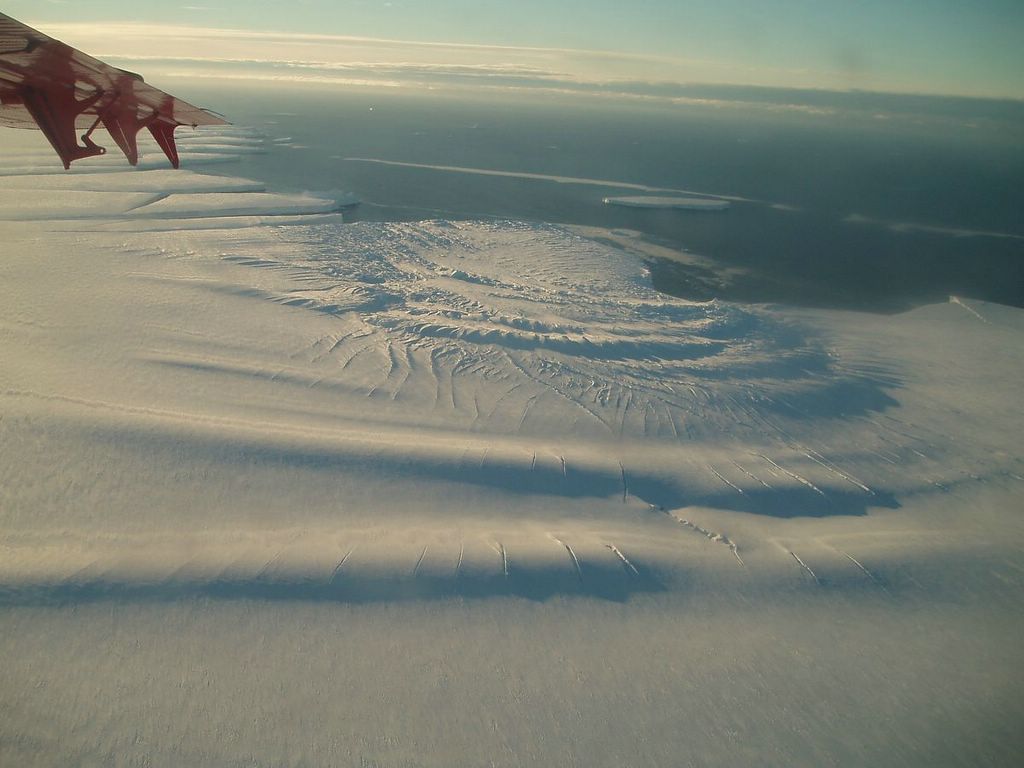
- When the Halloween crack cuts all the way across, the area of ice lost from the shelf will likely be at least 1700 km2 (660 square miles). That’s not a terribly large iceberg by Antarctic standards—probably not even making the top 20 list. But it may be the largest berg to break from the Brunt Ice Shelf since observations began in 1915. Scientists are watching to see if the loss will trigger the shelf to further change and possibly become unstable or break up.
- “The near-term future of Brunt Ice Shelf likely depends on where the existing rifts merge relative to the McDonald Ice Rumples,” said Joe MacGregor, a glaciologist at NASA’s Goddard Space Flight Center. “If they merge upstream (south) of the McDonald Ice Rumples, then it’s possible that the ice shelf will be destabilized.”
- The growing cracks have prompted safety concerns for people working on the shelf, particularly researchers at the British Antarctic Survey’s Halley Station. This major base for Earth, atmospheric, and space science research typically operates year-round, but has been closed down twice in recent years due to unpredictable changes in the ice. The station has also been rebuilt and relocated over the decades. The detailed image (Figure 109) shows the station’s location (Halley IV) until it was closed in 1992. In 2016-2017, the Halley VI station was relocated to a safer location (Halley VIa) upstream of the growing crack.
- Calving is a normal part of the life cycle of ice shelves, but the recent changes are unfamiliar in this area. The edge of the Brunt Ice Shelf has evolved slowly since Ernest Shackleton surveyed the coast in 1915, but it has been speeding up in the past several years.
- “We don’t have a clear picture of what drives the shelf’s periods of advance and retreat through calving,” said NASA/UMBC glaciologist Chris Shuman. “The likely future loss of the ice on the other side of the Halloween Crack suggests that more instability is possible, with associated risk to Halley VIa.”
• February 11, 2019: About 13 percent of the Alaskan landscape has changed in some way in recent decades. That’s the conclusion of a 2018 study led by Neal Pastick, who examined historical aerial photos and satellite images to identify areas of ecological change across the state. 56)
- “We set out to characterize all of these changes by using remote sensing data from the past 32 years,” said Pastick, a physical scientist and contractor to the U.S. Geological Survey Earth Resources Observation Science Center. “It’s striking how much change is happening, and what we can do with the Landsat satellites to link these changes into one cohesive story.”
- The most notable changes in Alaska include the browning of land from forest fires and the greening of the land as vegetation regrows. Pastick also documented vast areas of land affected by erosion, including segments of coastline that have dramatically changed shape.
- Warming temperatures have played a major role in the coastline retreat. Melting permafrost leaves the ground less stable and more prone to being washed away by heavy rains and pounding ocean waves. Rising temperatures cause the protective sea ice cover to disappear for longer periods each spring and summer, meaning waves and Arctic storms can more easily chew away at the coastline. No one lives along the receding coastline shown above, but coastal communities elsewhere in Alaska have had to make decisions about how to deal with failing infrastructure as permafrost melts and coastlines retreat.
- More work is needed in order to identify how the changing landscape will continue to affect communities, according to Pastick. He added: “I want to understand how these evolving systems might change in the future, and what that change means for people who live there.”
• February 11, 2019: Today marks the 5th anniversary of the launch of Landsat-8 from Vandenberg Air Force Base in California. A joint NASA and USGS mission, Landsat-8 adds to the longest continuous data record of Earth’s surface as viewed from space. Since launch, Landsat-8 has completed over 25,500 Earth orbits, traveled over 700 million miles, and contributed over 1.1 million scenes to the USGS Landsat archive. 57)
- Since 2013, Landsat 8 data has been cited in over 600 peer reviewed journal publications supporting studies from agriculture, forest and water quality/use/management, to natural disaster support, and mapping and monitoring land change, to name a few.
• February 10, 2019: With the International Energy Agency forecasting that the number of electric motor vehicles will skyrocket from about 3 million in 2018 to 125 million by 2030, it is a good bet that more of these vividly colored evaporation ponds will dot deserts in South America in the future. That’s because they are a key source of lithium. 58)
- Makers of electric vehicles, laptops, cell phones, and other gadgets rely heavily on lithium for rechargeable batteries. Lithium is also used in ceramics, glass, industrial grease, and medication. With 29 percent of the world’s reserves, Chile’s Salar de Atacama—an enclosed basin with no drainage outlets—is the world’s largest source of lithium. Nearby areas in Bolivia and Argentina also have large reserves.
- While the surface of the salar (Spanish for salt flat) is almost always dry, a large reserve of lithium-rich brine lurks below the surface of the ancient sea bed. A combination of snowmelt from nearby mountains and hydrothermal fluids associated with volcanic activity naturally replenishes the aquifer.
- As the number of ponds at Salar de Atacama increases over time to meet the rising demand for lithium, there are concerns and conflicts brewing about how much groundwater companies operating in this area are using.
• February 5, 2019: Two hundred million years ago, dinosaurs roamed the land that is now northwest Argentina. Today, those prehistoric reptiles linger as some of the world’s oldest and most pristine fossils—spanning 50 million years from when dinosaurs first appeared to when they rose to dominance in the Triassic era. 59)
- Like a South American version of Monument Valley in the United States, Talampaya Park is known for its 200-meter high red sandstone cliffs and 1,500-year-old rock carvings. The image of Figure shows a close-up view of the park in La Rioja province, where the aptly named herbivorous dinosaur Riojasaurus was discovered.
- Talampaya stands in stark contrast to the white and multicolor sediments of the Ischigualasto Provincial Park to the south. Ischigualasto is often called the Valle de la Luna (“Valley of the Moon”) because its unique and rugged terrain give an otherworldly appearance.
- Now a basin of sandstone and mudstone, Ischigualasto used to be a volcanically active floodplain with rivers and strong seasonal rainfall. About 230 million years ago, during the age of the dinosaurs, rock deposits filled the basin and fossilized the surrounding flora and fauna. In Ischigualasto, paleontologists have discovered a completely intact dinosaur skull of the Herrerasaurus, as well as the Eoraptor lunensis, one of the most primitive dinosaurs discovered to date.
- Today, the parks are arid scrub deserts located in the Argentine Monte, one of the driest regions in the country. Both parks are listed as UNESCO World Heritage sites because of their archaeological significance.
• February 2, 2019: For the first time in perhaps a decade, Mount Etna experienced a “flank eruption”—erupting from its side instead of its summit—on 24 December 2018. The activity was accompanied by 130 earthquakes occurring over three hours that morning. Mount Etna, Europe’s most active volcano, has seen periodic activity on this part of the mountain since 2013. 60)
- Ash spewing from the fissure cloaked adjacent villages and delayed aircraft from landing at the nearby Catania airport. Earthquakes occurred in the subsequent days after the initial eruption and displaced hundreds of people from their homes, according to news reports.
1) ”Marree Man,” NASA Earth Observatory, 29 December 2019, URL: https://earthobservatory.nasa.gov/images/146061/marree-man
2) ”Lanzarote’s Lunar-Like Landscape,” NASA Earth Observatory, Image of the Day for 25 December 2019, URL: https://earthobservatory.nasa.gov/images/146057/lanzarotes-lunar-like-landscape
3) ”Roads for Ships,” NASA Earth Observatory, Image of the Day for 24 December 2019, URL: https://earthobservatory.nasa.gov/images/146047/roads-for-ships
4) ”The Expansion of Shanghai,” NASA Earth Observatory, Image of the Day for 11 December 2019, URL: https://earthobservatory.nasa.gov/images/145968/the-expansion-of-shanghai
5) ”Sediment Sloshes in Solway Firth,” NASA Earth Observatory, 7 December 2019, URL: https://earthobservatory.nasa.gov/images/145958/sediment-sloshes-in-solway-firth
6) ”Satellites Track Status of Nation’s Food Supply,” NASA, 27 November 2019, URL: https://www.nasa.gov/feature/goddard/2019/landsat-data-maps-nation
7) ”All Eyes on Tonga’s Kingdom of Volcanoes,” NASA Earth Observatory, Image of the Day for 27 November 2019, URL: https://earthobservatory.nasa.gov/images/145919/all-eyes-on-tongas-kingdom-of-volcanoes
8) ”The Oysters of Tongyeong,” NASA Earth Observatory, Image of the Day for 25 November 2019, URL: https://earthobservatory.nasa.gov/images/145903/the-oysters-of-tongyeong
9) ”The Highest Settlement in the World,” NASA Earth Observatory, Image of the Day for 15 November 2019, URL: https://earthobservatory.nasa.gov/images/145864/the-highest-settlement-in-the-world
10) ”40 years of Landsat in Australia- The Alice Springs Ground Station,” Geoscience Australia, 11 November 2019, URL: https://www.ga.gov.au/news-events/features/40-years-of-landsat-in-australia
11) ”The Many Meanders of the Juruá,” NASA Earth Observatory, Image of the Day for 13 November 2019, URL: https://earthobservatory.nasa.gov/images/145819/the-many-meanders-of-the-jurua
12) ”Retreat Begins at Taku Glacier,” NASA Earth Observatory, Image of the Day for 5 November 2019, URL: https://earthobservatory.nasa.gov/images/145830/retreat-begins-at-taku-glacier
13) ”Oleshky Sands,” NASA Earth Observatory, Image of the Day for 31 October 2019, URL: https://earthobservatory.nasa.gov/images/145801/oleshky-sands?src=eoa-iotd
14) ”Strong Gusts Spread the Kincade Fire,” NASA Earth Observatory, Image of the Day for 30 October 2019, URL: https://earthobservatory.nasa.gov/images/145793/strong-gusts-spread-the-kincade-fire
15) ”India’s Largest Salt Producer,” NASA Earth Observatory, Image of the Day for 21 October 2019, URL: https://earthobservatory.nasa.gov/images/145756/indias-largest-salt-producer?src=eoa-iotd
16) ”Assateague on the Move,” NASA Earth Observatory, 9 October 2019, URL: https://earthobservatory.nasa.gov/images/145695/assateague-on-the-move
17) ”The Long Bridge to “Silk City”,” NASA Earth Observatory, Image of the Day for 20 September 2019, URL: https://earthobservatory.nasa.gov/images/145624/the-long-bridge-to-silk-city
18) ”Drought Reveals Lost “Spanish Stonehenge”,” NASA Earth Observatory, Image of the Day for 19 September 2019, URL: https://earthobservatory.nasa.gov/images/145619/drought-reveals-lost-spanish-stonehenge
19) ”Cameron Ridge,” NASA Earth Observatory, Image of the Day for17 September 2019, URL: https://earthobservatory.nasa.gov/images/145607/cameron-ridge?src=eoa-iotd
20) ”A Bloom of Nitrogen-Fixing Bacteria,” NASA Earth Observatory, Image of the Day for 16 September 2019, URL: https://earthobservatory.nasa.gov/images/145610/a-bloom-of-nitrogen-fixing-bacteria?src=eoa-iotd
21) ”Malaspina on the Move,” NASA Earth Observatory, 11 September 2019, URL: https://earthobservatory.nasa.gov/images/145574/malaspina-on-the-move
22) ”Nearing the Limit of Retreat,” NASA Earth Observatory, Image of the Day for 29 August 2019, URL: https://earthobservatory.nasa.gov/images/145525/nearing-the-limit-of-retreat?src=eoa-iotd
23) ”Landmarks of the Pacific Crest Trail,” NASA Earth Observatory, Image of the day for 28 August 2019, URL: https://earthobservatory.nasa.gov/images/145504/landmarks-of-the-pacific-crest-trail?src=eoa-iotd
24) ”A Raft of Rock,” NASA Earth Observatory, Image of the day for 23 August 2019, URL: https://earthobservatory.nasa.gov/images/145490/a-raft-of-rock?src=eoa-iotd
25) ”Okjökull Remembered,” NASA Earth Observatory, Image of the Day for 9 August 2019, URL: https://earthobservatory.nasa.gov/images/145439/okjokull-remembered?src=eoa-iotd
26) ”Iceland’s Raging Rivers,” NASA Earth Observatory, Image of the Day for 6 August 2019, URL: https://earthobservatory.nasa.gov/images/145408/icelands-raging-rivers
27) ”Dreaming in the Mojave Desert,” NASA Earth Observatory, 6 August 2019, URL: https://earthobservatory.nasa.gov/images/145400/dreaming-in-the-mojave-desert
28) ”Getting Saltier,” NASA Earth Observatory, Image of the Day for 31 July 2019, URL: https://earthobservatory.nasa.gov/images/145373/getting-saltier?src=eoa-iotd
29) ”South Africa’s Largest Open-Pit Mine,” NASA Earth Observatory, Image of the Day for 30 July 2019, URL: https://earthobservatory.nasa.gov/images/145366/south-africas-largest-open-pit-mine?src=eoa-iotd
30) ”Hammerhead Horsts on the Makran Coast,” NASA Earth Observatory, Image of the Day for 24 July 2019, URL: https://earthobservatory.nasa.gov/images/145350/hammerhead-horsts-on-the-makran-coast
31) ”Green Space is Good for Mental Health,” NASA Earth Observatory, Image of the Day for 17 July 2019, URL: https://earthobservatory.nasa.gov/images/145305/green-space-is-good-for-mental-health?src=eoa-iotd
32) Kristine Engemann, Carsten Bøcker Pedersen, Lars Arge, Constantinos Tsirogiannis, Preben Bo Mortensen, and Jens-Christian Svenning, ”Residential green space in childhood is associated with lower risk of psychiatric disorders from adolescence into adulthood,” PNAS (Proceedings of the National Academy of Sciences of the United States of America), 12 March 2019, Vol. 116, No 11, pp: 5188-5193, https://doi.org/10.1073/pnas.1807504116, URL: https://www.pnas.org/content/pnas/116/11/5188.full.pdf
33) ”Kolyma’s Annual Purge,” NASA Earth Observatory, Image of the Day for 14 July 2019, URL: https://earthobservatory.nasa.gov/images/145272/kolymas-annual-purge?src=eoa-iotd
34) ”The Sea Takes Back a Baby Island-A tiny island birthed by an earthquake and a mud volcano has faded into the sea,” NASA Earth Observatory, Image of the Day for July 5, 2019, URL: https://earthobservatory.nasa.gov/images/145265/the-sea-takes-back-a-baby-island?src=eoa-iotd
35) ”Major Greenland Glacier Is Growing,” NASA Earth Observatory, 18 June 2019, URL: https://earthobservatory.nasa.gov/images/145185/major-greenland-glacier-is-growing?src=eoa-iotd
36) ”Cold Water Currently Slowing Fastest Greenland Glacier,” NASA/JPL-Caltech, 25 March 2019, URL: https://www.jpl.nasa.gov/news/news.php?feature=7356
37) ”Solar-Powered China,” NASA Earth Observatory, 17 June 2019, URL: https://earthobservatory.nasa.gov/images/145159/solar-powered-china
38) ”Eerie Green Swirls of Lake Khanka,” NASA Earth Observatory, 12 June 2019, URL: https://earthobservatory.nasa.gov/images/145073/eerie-green-swirls-of-lake-khanka
39) Emil Cherrington, ”On the Ground in Belize to Improve How Satellites “See” Water Quality from Space,” NASA Earth Observatory, 3 June 2019, URL: https://earthobservatory.nasa.gov/blogs/fromthefield/2019/06/03/on-the-ground-in-belize-to-improve-how-satellites-see-water-quality-from-space/
40) ”Surging Glacier Creates a New Lake,” NASA Earth Observatory, 15 May 2019, URL: https://earthobservatory.nasa.gov/images/145038/surging-glacier-creates-a-new-lake?src=eoa-iotd
41) ”Reservoir Swells Upstream of Mosul,” NASA Earth Observatory, 8 May 2019, URL: https://earthobservatory.nasa.gov/images/145010/reservoir-swells-upstream-of-mosul
42) ”20 Years of NASA Earth Observatory,” NASA Earth Observatory, 7 May 2019, URL: https://earthobservatory.nasa.gov/features
43) https://earthobservatory.nasa.gov/topic/videos
44) ”Pushing Limits at Armstrong Flight Research Center,” NASA Earth Observatory, Image of the Day for 23 April 2019, URL: https://earthobservatory.nasa.gov/images/144861/pushing-limits-at-armstrong-flight-research-center
45) ”A Fire Surrounded by Ice,” NASA Earth Observatory, 10 April 2019, URL: https://earthobservatory.nasa.gov/images/144803/a-fire-surrounded-by-ice?src=eoa-iotd
46) ”History on a Hill,” NASA Earth Observatory, 2 April 2019, URL: https://earthobservatory.nasa.gov/images/144736/history-on-a-hill
47) ”A Honking, Fluttering Spectacle,” NASA Earth Observatory, Image of the day for 26 March 2019, URL: https://earthobservatory.nasa.gov/images/144680/a-honking-fluttering-spectacle
48) ”Icy Floodwaters Grind Through Iowa,” NASA Earth Observatory, 19 March 2019, URL: https://earthobservatory.nasa.gov/images/144696/icy-floodwaters-grind-through-iowa?src=eoa-iotd
49) ”Satellites Find Greener Pastures,” NASA Earth Observatory, 13 March 2019, URL: https://earthobservatory.nasa.gov/images/144654/satellites-find-greener-pastures
50) ”Jupiter or Earth?,” NASA Earth Observatory, 11 March 2019, URL: https://earthobservatory.nasa.gov/images/144643/jupiter-or-earth?src=eoa-iotd
51) Flooding on the Russian River,” NASA Earth Observatory, 6 March 2019, URL: https://earthobservatory.nasa.gov/images/144619/flooding-on-the-russian-river
52) ”Savage South Georgia,” NASA Earth Observatory, 4 March 2019, URL: https://earthobservatory.nasa.gov/images/144476/savage-south-georgia
53) ”Australia’s Disappearing Lakes Disappear Even More,” NASA Earth Observatory, Image of the day for 26 February 2019, URL: https://earthobservatory.nasa.gov/images/144577/australias-disappearing-lakes-disappear-even-more
54) ”Brazil’s Carajás Mines,” NASA Earth Observatory, Image of the day for 23 February 2019, URL: https://earthobservatory.nasa.gov/images/144457/brazils-carajas-mines
55) ”Countdown to Calving at Brunt Ice Shelf,” NASA Earth Observatory, Image of the day for20 February 2019, URL: https://earthobservatory.nasa.gov/images/144563/countdown-to-calving-at-brunt-ice-shelf
56) ”Alaska in Flux: Slumping Coastlines,” NASA Earth Observatory, Image of the day for 11 February 2019, URL: https://earthobservatory.nasa.gov/images/144527/alaska-in-flux-slumping-coastlines
57) ”NASA and USGS Celebrate 5 Year Launch Anniversary of Landsat 8,” USGS, 8 February 2019, URL: https://www.usgs.gov/landsat-missions/february-8-2018-nasa-and-usgs-celebrate-5-year-launch-anniversary-landsat-8
58) ”Where Batteries Begin,” NASA Earth Observatory, Image of the day for 9 February 9 2019, URL: https://earthobservatory.nasa.gov/images/144393/where-batteries-begin
59) ”Time Traveling to the Triassic,” NASA Earth Observatory, Image of the day for 5 February 2019, URL: https://earthobservatory.nasa.gov/images/144431/time-traveling-to-the-triassic
60) ”Etna Awakens on its Side,” NASA Earth Observatory, Image of the day for 2 February 2019, URL: https://earthobservatory.nasa.gov/images/144493/etna-awakens-on-its-side
References Back to top