Terra (EOS/AM-1)
EO
Multiple direction/polarisation radiometers
Atmosphere
Ocean
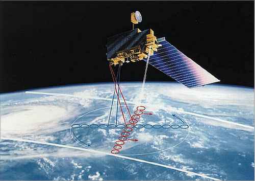
Launched in December 1999, Terra (formerly known as EOS/AM-1) is a joint mission within NASA’s ESE (Earth Science Enterprise) program between the US, Japan and Canada. With an original design life of six years, the operation has been extended to continue to provide an extensive variety of valuable data on Earth’s atmosphere, land surface, ocean and cryosphere.
Quick facts
Overview
| Mission type | EO |
| Agency | NASA, CSA, METI |
| Mission status | Operational (extended) |
| Launch date | 18 Dec 1999 |
| Measurement domain | Atmosphere, Ocean, Land, Snow & Ice |
| Measurement category | Cloud type, amount and cloud top temperature, Atmospheric Temperature Fields, Cloud particle properties and profile, Ocean colour/biology, Aerosols, Multi-purpose imagery (ocean), Radiation budget, Multi-purpose imagery (land), Surface temperature (land), Vegetation, Albedo and reflectance, Surface temperature (ocean), Atmospheric Humidity Fields, Ozone, Trace gases (excluding ozone), Landscape topography, Sea ice cover, edge and thickness, Snow cover, edge and depth, Atmospheric Winds, Ice sheet topography |
| Measurement detailed | Cloud top height, Ocean imagery and water leaving spectral radiance, Aerosol absorption optical depth (column/profile), Ocean chlorophyll concentration, Downward long-wave irradiance at Earth surface, Cloud cover, Cloud optical depth, Aerosol optical depth (column/profile), Cloud type, Cloud ice content (at cloud top), Color dissolved organic matter (CDOM), Cloud imagery, Land surface imagery, Upward short-wave irradiance at TOA, Upward long-wave irradiance at TOA, Cloud drop effective radius, Aerosol effective radius (column/profile), Fire temperature, Vegetation type, Fire fractional cover, Earth surface albedo, Downwelling (Incoming) solar radiation at TOA, Short-wave Earth surface bi-directional reflectance, Leaf Area Index (LAI), Land cover, Atmospheric specific humidity (column/profile), O3 Mole Fraction, Atmospheric temperature (column/profile), Land surface temperature, Sea surface temperature, Land surface topography, Ocean suspended sediment concentration, Sea-ice cover, Snow cover, Cloud top temperature, Normalized Differential Vegetation Index (NDVI), Wind profile (horizontal), Sea-ice thickness, Atmospheric stability index, Photosynthetically Active Radiation (PAR), Fraction of Absorbed PAR (FAPAR), CO Mole Fraction, Sea-ice sheet topography, Downward short-wave irradiance at Earth surface, Long-wave Earth surface emissivity, Diffuse attenuation coefficient (DAC), Upwelling (Outgoing) long-wave radiation at Earth surface, Short-wave cloud reflectance |
| Instruments | CERES, MODIS, ASTER, MOPITT, MISR |
| Instrument type | Multiple direction/polarisation radiometers, Imaging multi-spectral radiometers (vis/IR), High resolution optical imagers, Earth radiation budget radiometers, Atmospheric chemistry |
| CEOS EO Handbook | See Terra (EOS/AM-1) summary |
Summary
Mission Capabilities
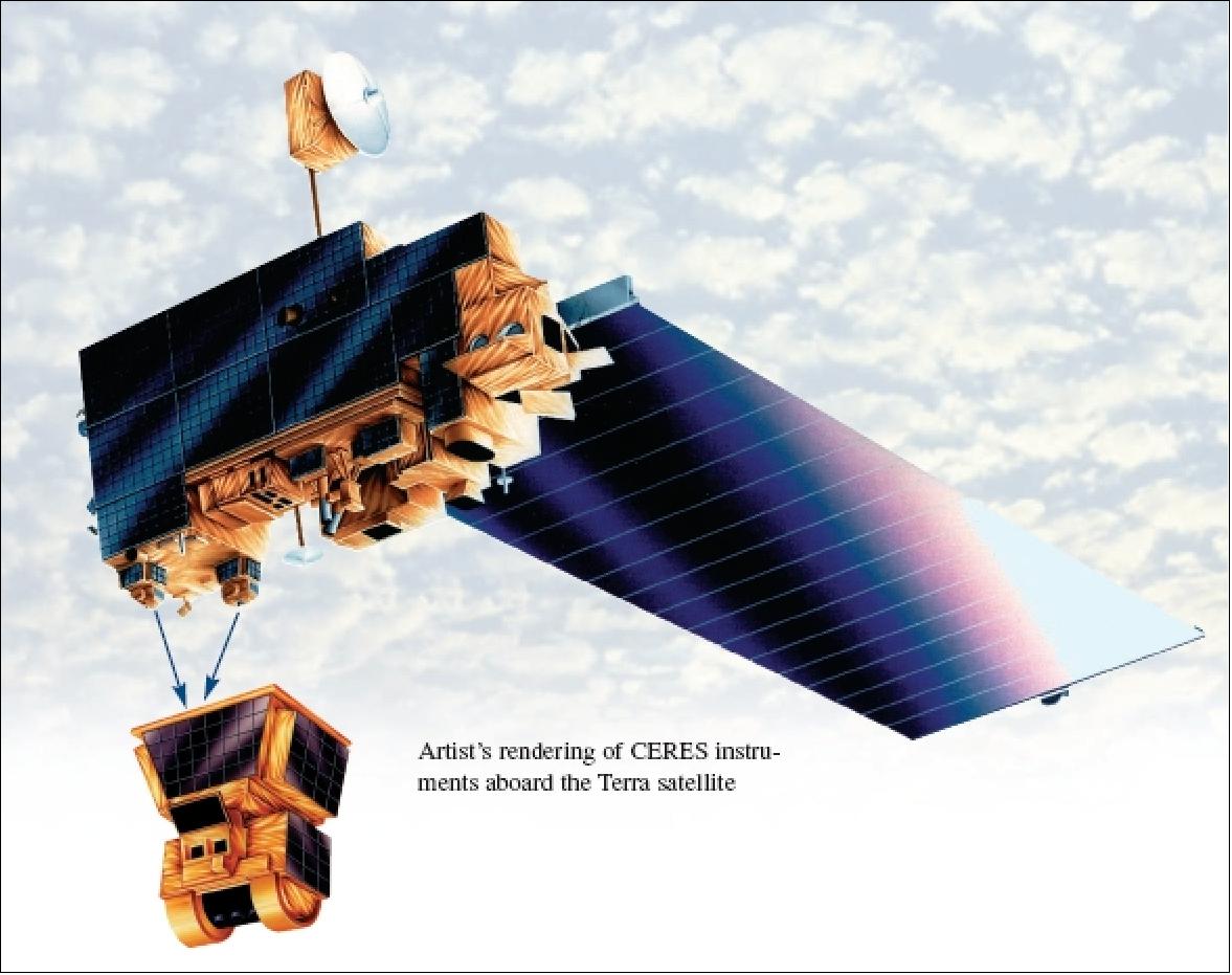
Terra features five onboard instruments, each with varying imaging capabilities for specific functions; ASTER, CERES, MISR, MODIS and MOPITT.
Developed in Japan, ASTER (Advanced Spaceborne Thermal Emission and Reflection Radiometer) consists of three separate subsystems to provide high-resolution multispectral imagery of the Earth’s surface and clouds. Analysis of this data allows for better understanding of the physical processes that affect climate change. The CERES (Clouds and the Earth’s Radiant Energy System) instrument, designed by NASA, is used for long-term measurement of the Earth’s radiation budget and atmospheric radiation from the top of the atmosphere to the surface.
The MISR (Multi-angle Imaging SpectroRadiometer) was developed by NASA’s Jet Propulsion Lab with the objective to provide multiple-angle continuous sunlight coverage of the Earth. It uses nine high resolution cameras to provide global maps of planetary and surface albedo, aerosols and vegetation properties. These datasets can subsequently be used to monitor global and regional trends in radiatively optical properties of natural and anthropogenic aerosols. Developed by NASA’s Goddard Space Flight Centre, MODIS (Moderate-Resolution Imaging Spectroradiometer) provides global data on four discipline groups: atmosphere, land, oceans and calibration. The final instrument onboard is MOPITT (Measurement of Pollution in the Troposphere) which is the first satellite sensor to use gas correlation spectroscopy. Designed by the Canadian Space Agency (CSA) and built by COM DEV, it is primarily used for measurement of the tropospheric chemistry in the atmosphere.
Performance Specifications
ASTER images in 14 bands in the shortwave infrared (SWIR), visible to near infrared (VNIR) and thermal infrared (TIR) regions. These each have a swath width of 60 km and a ground resolution of 15 m, 30 m and 90 m respectively. To measure Earth-emitted radiation and reflected sunlight, CERES uses two identical scanners that perform limb-to-limb scanning to observe longwave and shortwave infrared radiation at a spatial resolution of 10-20 km. MISR features nine onboard cameras which each image four spectral bands at a ground sampling distance of 275 m, 550 m or 1100 m, and together cover a swath of 360 km. Similarly, MODIS images 36 discrete bands with corresponding spatial resolutions of 250 m, 500 m and 1000 m used for land/cloud boundaries, land/cloud properties and complex land/cloud/ocean features respectively. Using 10 pixels in parallel along track it covers a large swath of 2300 km x 10 km. MOPITT uses eight channels, each with a spectral band constituent of carbon monoxide or methane thermal/solar, to observe how these gases interact with the surface, ocean and biomass systems. The instrument covers a swath width of 616 km at a spatial resolution of 22 x 22 km.
Terra undergoes a sun-synchronous circular orbit, at an altitude of 705 km and an inclination of 98.5°. It has a period of 99 minutes and a repeat cycle of 16 days.
Space and Hardware Components
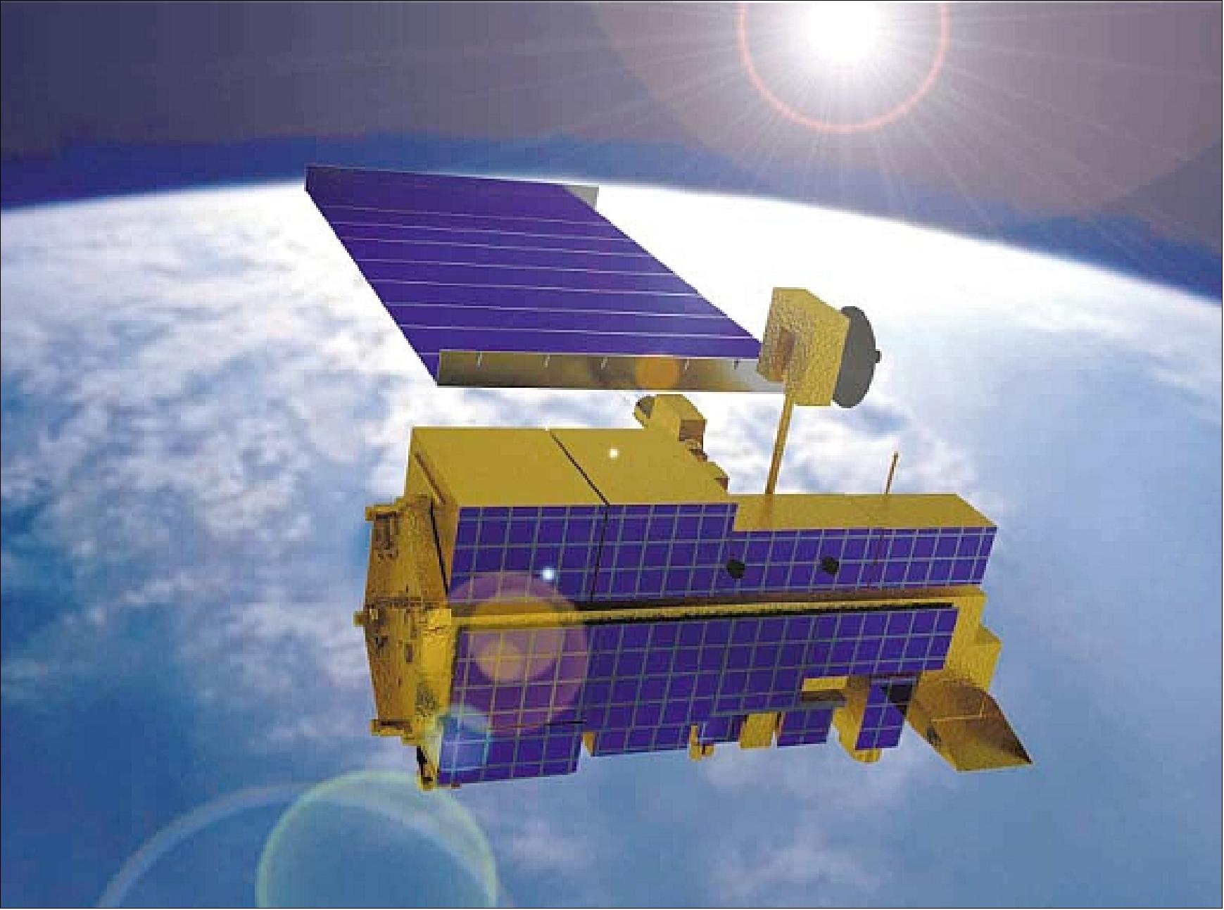
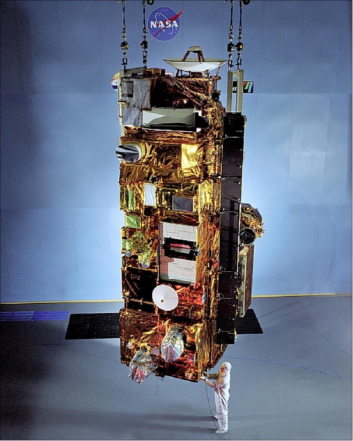
Terra features a three-axis stabilised spacebus developed by Lockheed Martin Missiles and Space (LMMS) with a truss-like primary structure. A large single-wing, rotating solar array maximises power generation. The primary telemetry data transmission is via a Tracking & Data Relay Satellite (TDRS) system which utilises Ku-band, S-band and X-band transmission. A TDRS Onboard Navigation System (TONS) performs orbit determination to estimate Terra’s velocity, drag coefficient and master oscillator frequency bias. Developed with an initial design life of six years, the spacecraft has a total launch mass of 5190 kg which includes an onboard payload mass of 1155 kg.
Terra Mission (EOS/AM-1)
Spacecraft Launch Mission Status Sensor Complement EOS References
Terra (formerly known as EOS/AM-1) is a joint Earth observing mission within NASA's ESE (Earth Science Enterprise) program between the United States, Japan, and Canada. The US provided the spacecraft, the launch, and three instruments developed by NASA (CERES, MISR, MODIS). Japan provided ASTER and Canada MOPITT. The Terra spacecraft is considered the flagship of NASA's EOS (Earth Observing Satellite) program. In February 1999, the EOS/AM-1 satellite was renamed by NASA to “Terra”. 1) 2) 3) 4)
The objective of the mission is to obtain information about the physical and radiative properties of clouds (ASTER, CERES, MISR, MODIS); air-land and air-sea exchanges of energy, carbon, and water (ASTER, MISR, MODIS); measurements of trace gases (MOPITT); and volcanology (ASTER, MISR, MODIS). The science objectives are:
• To provide the first global and seasonal measurements of the Earth system, including such critical functions as biological productivity of the land and oceans, snow and ice, surface temperature, clouds, water vapor, and land cover;
• To improve the ability to detect human impacts on the Earth system and climate, identify the “fingerprint” of human activity on climate, and predict climate change by using the new global observations in climate models;
• To help develop technologies for disaster prediction, characterization, and risk reduction from wildfires, volcanoes, floods, and droughts
• To start long-term monitoring of global climate change and environmental change.
Complemented by aircraft and ground-based measurements, Terra data will enable scientists to distinguish between natural and human-induced changes.
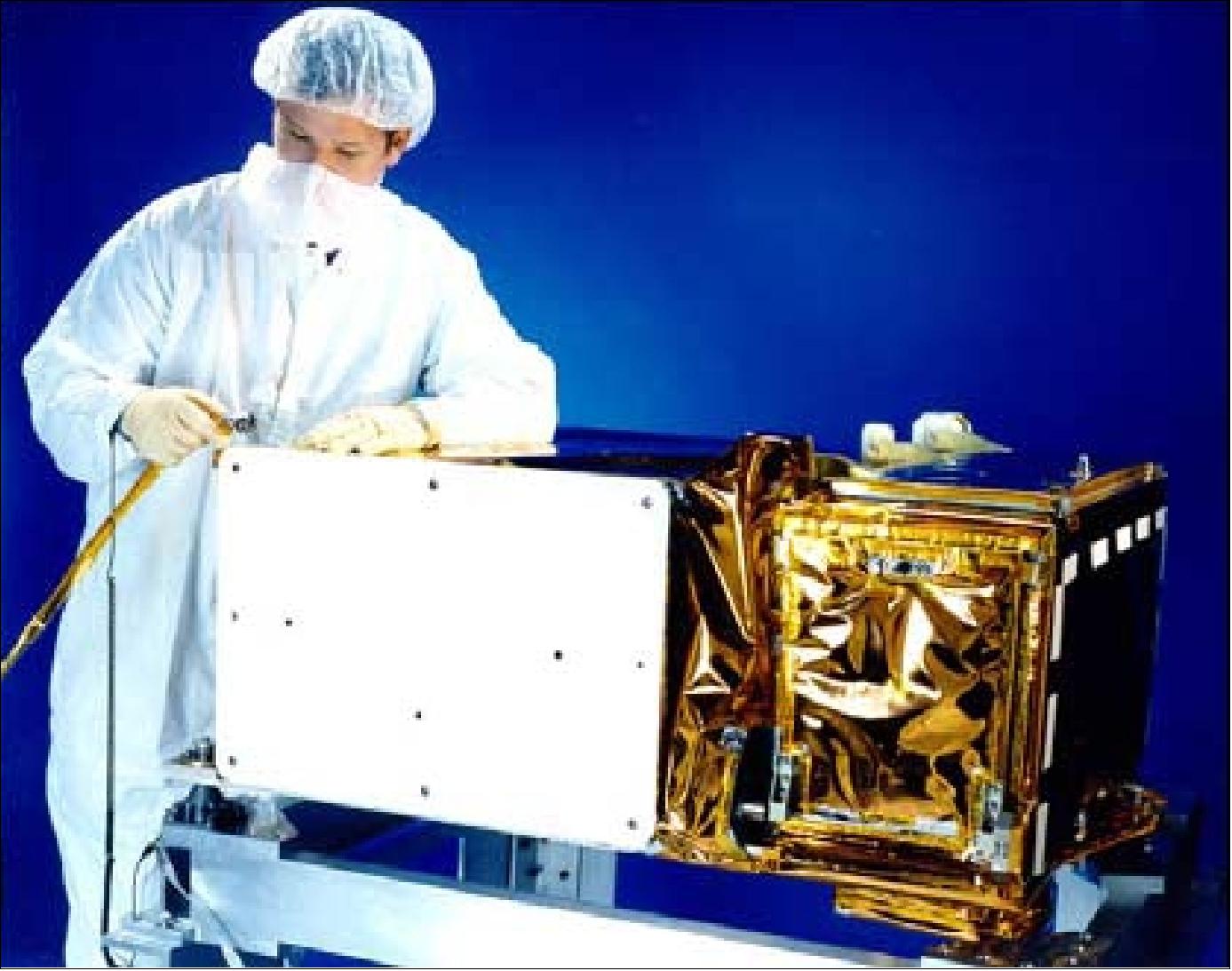
Spacecraft
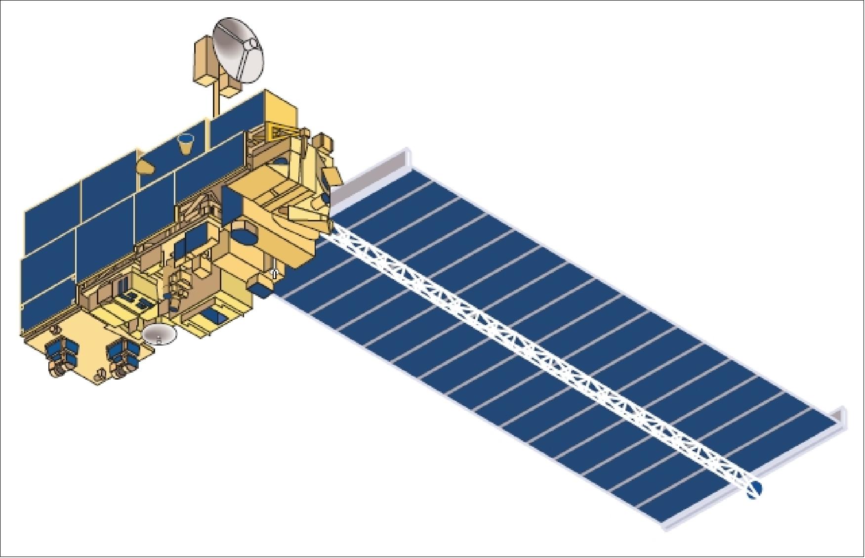
Terra consists of a spacecraft bus built by Lockheed Martin Missiles and Space (LMMS) in Valley Forge, PA. The spacecraft is constructed with a truss-like primary structure built of graphite-epoxy tubular members. This lightweight structure provides the strength and stiffness needed to support the spacecraft throughout its various mission phases. The zenith face of the spacecraft is populated with equipment modules (EMs) housing the various spacecraft bus components. The EMs are sized and partitioned to facilitate pre-launch integration and test of the spacecraft.
EPS (Electrical Power Subsystem): A large single-wing solar array (size of 9 m x 5 m = 45 m2), deployed on the sunlit side of the spacecraft, maximizes both its power generation capability and the cold-space FOV (Field of View) available to instrument and equipment module radiators. The average power of the satellite is 2.53 kW provided by a GaAs/Ge solar array (max of 7.5 kW @ 120 V at BOL). The solar array is based on on a prototype lightweight flexible blanket solar array technology developed by TRW (use of single-junction GaAs/Ge photovoltaics). A coilable mast is used for the deployment of the solar array. The Terra spacecraft represents the first orbiting application of a 120 VDC high voltage spacecraft electrical power system implemented by NASA. A PDU (Power Distribution Unit) has been designed to provide 120 DC (±4%) under any load conditions. This regulated voltage, in turn, is achieved via a sequential shunt unit (SSU) and the 2 BCDUs. A NiH2 (nickel hydrogen) battery is used (54 cells series connected) to provide power during eclipse phases of the orbit. 5) 6) 7)
GN&C (Guidance Navigation and Control) subsystem: Terra is a three-axis stabilized design with a single rotating solar array. The GN&C subsystem is made up of sensors, actuators, an ACE (Attitude Control Electronics) unit, and software. A three-channel IRU (Inertial Reference Unit) determines body rates in all control modes. Solid-state star trackers provide fine attitude updates, processed by a Kalman filter to maintain precise 3-axis inertial knowledge. A 3-axis magnetometer senses the Earth's geomagnetic field, primarily for magnetic unloading of reaction wheels, but also as a sensor to determine an attitude failure during a deep space calibration maneuver. 8)
The backup sensors include an ESA (Earth Sensor Assembly) for roll and pitch sensing, and coarse sun sensors for pitch and yaw sensing of the sun line relative to the solar array. A fine sun sensor is used in the event that one star tracker fails or during the backup stellar acquisition mode. In addition to these sensors, a gyro-compassing computation is performed for backup yaw attitude determination.
A reaction wheel assembly provides primary attitude control. During normal mode, a wheel speed controller is available to bias the wheel speeds at a range that avoids zero rpm crossings (stagnation point). Magnetic torquer rods regulate the wheel momentum to < 25% capacity in four-wheel mode and < 50% capacity in the three-wheel mode (backup mode). Thrusters are used for attitude control during all velocity change maneuvers and for backup attitude control and wheel momentum unloading.
GN&C is a fault-tolerant system that includes an FDIR (Fault Detection, Isolation and Recovery) capability unique to each of the different operational control modes. If an attitude fault is detected, FDIR transfers all control functions to the ACE unit configured to use all redundant hardware. Once in safe mode, FDIR is disabled.
Sensor component | Units | Manufacturer/model | Mission heritage |
Solid State Star Tracker (SSST) | 2 | BATC / CT-601 | MSX, XTE |
Earth Sensor Assembly) (ESA) | 2 | Ithaco / conical scanning | UARS |
Coarse Sun Sensor (CSS) | 2 | Adcole / 42060 | UARS |
Fine Sun Sensor (FSS) | 1 | Adcole / 42070 | TOPEX |
Three Axis Magnetometer (TAM) | 2 | NASA/GSFC | EUVE, UARS |
Inertial Reference Unit (IRU) | 2 | Kearfott / SKIRU-DII | XTE |
|
|
|
|
Actuator component | Units | Manufacturer/model | Heritage |
Reaction Wheel Assembly (RWA) | 4 | Honeywell / EOS-AM | Similar to EUVE |
Magnetic Torquer Rod (MTR) | 3 | Ithaco / TR500CFR | EUVE |
Attitude Control Thruster | 6 (x 2) | Olin Aerospace (Primex) |
|
Delta-v thruster | 2 (x 2) | Olin Aerospace (Primex) |
|
The design life of the Terra spacecraft is six years. The spacecraft bus is of size of 6.8 m (length) x 3.5 m (diameter) and has a total launch mass of 5,190 kg. The total payload mass is 1155 kg.
RF communications: The primary Terra telemetry data transmissions are via TDRS (Tracking & Data Relay Satellite) system. A steerable HGA (High Gain Antenna) and associated electronics are mounted on a deployed boom extending from the zenith side of the spacecraft. This location maximizes the amount of time available for TDRS communications via this antenna without obstruction by other pads of the spacecraft. Emergency communication is done via the nadir or zenith omni antenna. Command and engineering telemetry data are transmitted in S-band. The science data recorded onboard are transmitted via Ku-band at 150 Mbit/s. The nominal mode of operation is to acquire two 12 minute TDRSS contacts per orbit. During each TDRSS contact, both S-band and Ku-band transmission is being used.
The average data rate of the payload is 18.545 Mbit/s (109 Mbit/s peak); onboard recorders for data collection of one orbit. Mission operations are performed at GSFC. 9)
Broadcast of data: Besides Ku-band and S-band communication, Terra is also capable of downlinking science data via X-band. The X-band communication can be operated in three different modes, Direct Broadcast (DB), Direct Downlink (DDL) and Direct Playback (DP). DB and DDL is used to directly transmit real-time MODIS and ASTER science data respectively to users.
The DAS (Direct Access System) provides a backup option for direct transmission in X-band. DAS supports transmission of data to ground stations of qualified EOS users around the world. These users fall into three categories:
- EOS team participants and interdisciplinary scientists
- International meteorological and environmental agencies
- International partners who require data from their EOS instruments
Launch
The launch of the Terra spacecraft took place on Dec. 18, 1999 from VAFB, CA, on an Atlas-Centaur IIAS rocket.
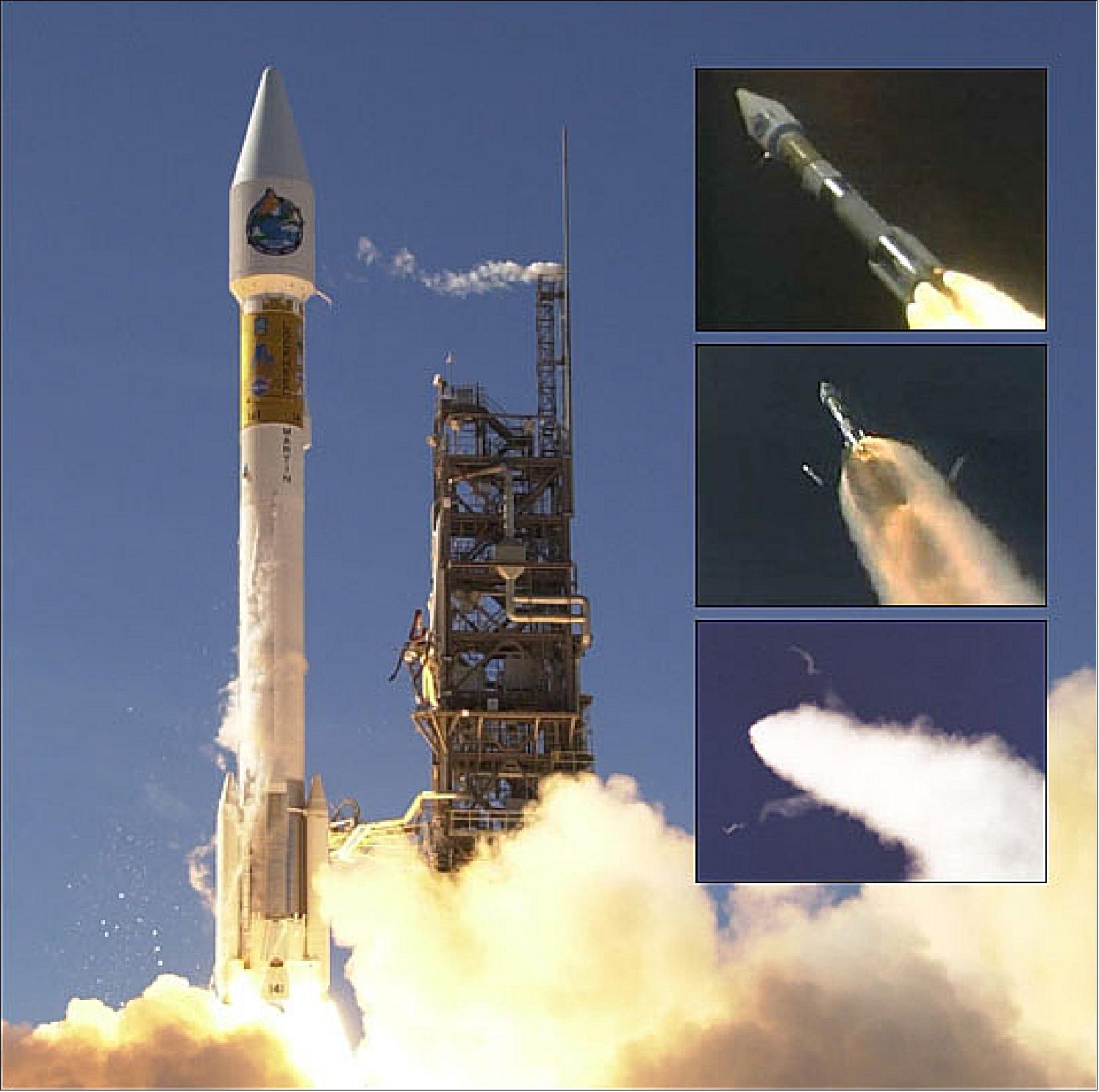
Orbit: Sun-synchronous circular orbit, altitude = 705 km, inclination = 98.5º, period = 99 minutes (16 orbits per day, 233 orbit repeat cycles). The descending nodal crossing is at 10:30 AM.
Orbit determination is performed by TONS (TDRS Onboard Navigation System) which estimates Terra's position and velocity, drag coefficient, and master oscillator frequency bias. TONS is updated by Doppler measurements at the spacecraft's receivers and provides the attitude control software with a desired pointing ephemeris. Ground-based orbital elements are uplinked daily for backup navigation.
As of March 1, 2001, the Landsat-7, EO-1, SAC-C and Terra satellites are flying the so-called “morning constellation” or “morning train” (a loose formation demonstration of a single virtual platform). There is 1 minute separation between Landsat-7 and EO-1, a 15 minute separation between EO-1 and SAC-C, and a 1 minute separation between SAC-C and Terra. The objective is to compare coincident observations (imagery) from various instruments (synergistic effects). 10)
• November 19, 2021: Terra's Orbital Drift 11)
Note: As of April 2022, the previously large Terra file has been split into four files, to make the file handling manageable for all parties concerned, in particular for the user community.
• This article covers the Terra mission and its imagery in the period 2022, in addition to some of the mission milestones.
• Terra status and imagery in the period 2021-2020
• Terra status and imagery in the period 2019
• Terra status and imagery in the period 2018-1999
Mission Status
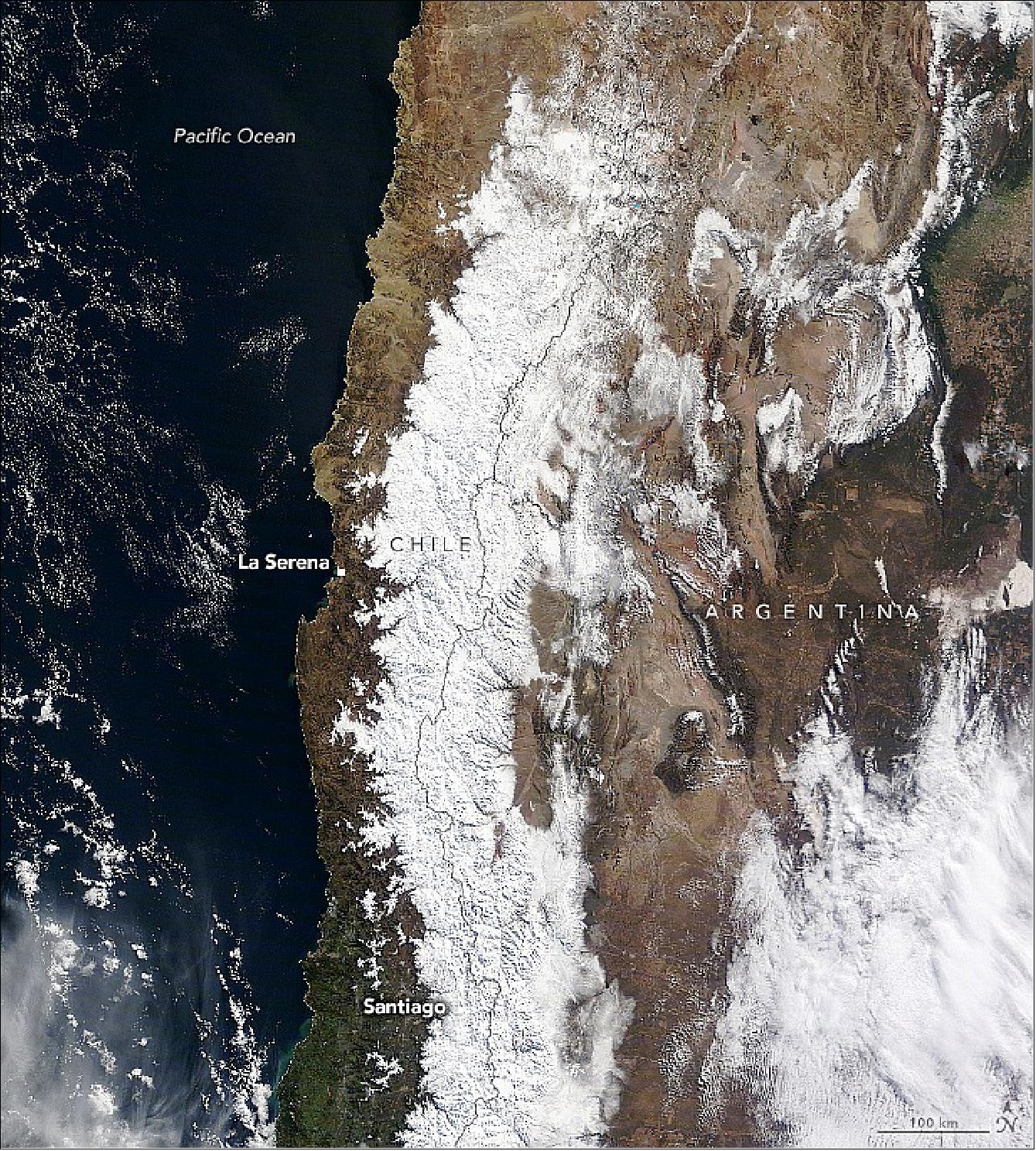
• July 20, 2022: As extreme summer heatwaves deepened droughts and fueled wildfires in the Northern Hemisphere, winter storms brewed south of the equator. In July 2022, back-to-back weather systems eased rainfall deficits in central Chile and added to the snowpack atop the Andes—a critical reserve of water for the coming summer. 12) The storms were the result of a blocking anticyclone atmospheric pattern near the Antarctic Peninsula that steered several extratropical cyclones toward Chile. On July 7, the coastal city of La Serena had a year-to-date rainfall deficit of about 80 percent (compared to the mean from 1990-2020). The storms delivered 8 centimeters (3 inches) of rain, bringing the city to a 64 percent surplus. Farther inland, Santiago’s rainfall deficit improved from 70 percent to 27 percent. The Terra Satellite was used to document these conditions.
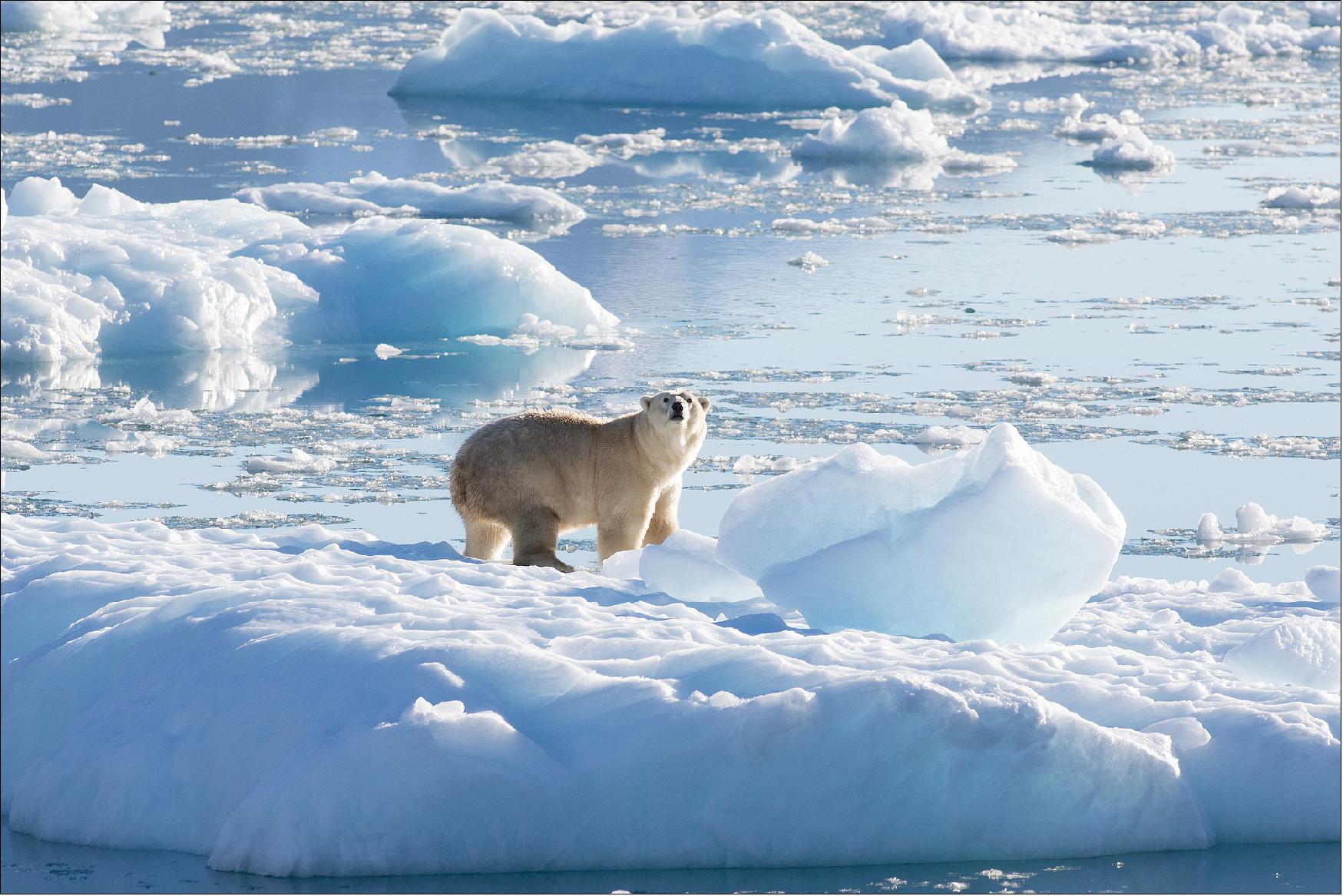
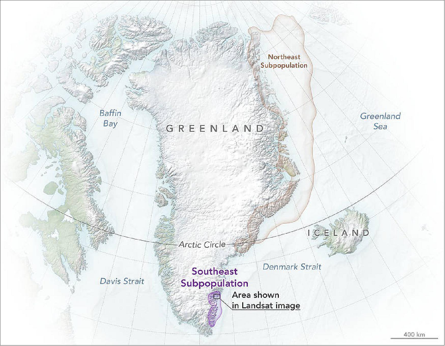
• June 16, 2022: Greenland’s fjords harbor a unique group of polar bears that rely on glacial ice, a NASA-funded study reports today in Science. 13) Polar bears throughout the Arctic depend on sea ice as a platform for hunting seals. But in Southeast Greenland, researchers found that bears survive for most of the year in fjords by relying on ice melanges, a mix of sea ice and pieces of glacial ice that is carved off of marine-terminating glaciers. They also used the Moderate Resolution Imaging Spectroradiometer instruments (MODIS) aboard NASA’s Terra and Aqua satellites and NSIDC data to document the fjord and offshore sea ice environment. Their findings revealed that the Southeast Greenland bears are cut off from sea ice two-thirds of the year, and supplement their hunting by using freshwater ice slabs, which routinely break off from the Greenland Ice Sheet and coastal glaciers. The team also used the MODIS instrument and data from the National Snow and Ice Data Center (NSIDC) to document the conditions in the fjords and the offshore sea ice environment. They found that southeastern polar bears are cut off from sea ice for two-thirds of the year. From late May until the sea ice returns in February, the bears hunt from atop the pieces of broken glacial ice floating at the front of glaciers—a mixture known as mélange.
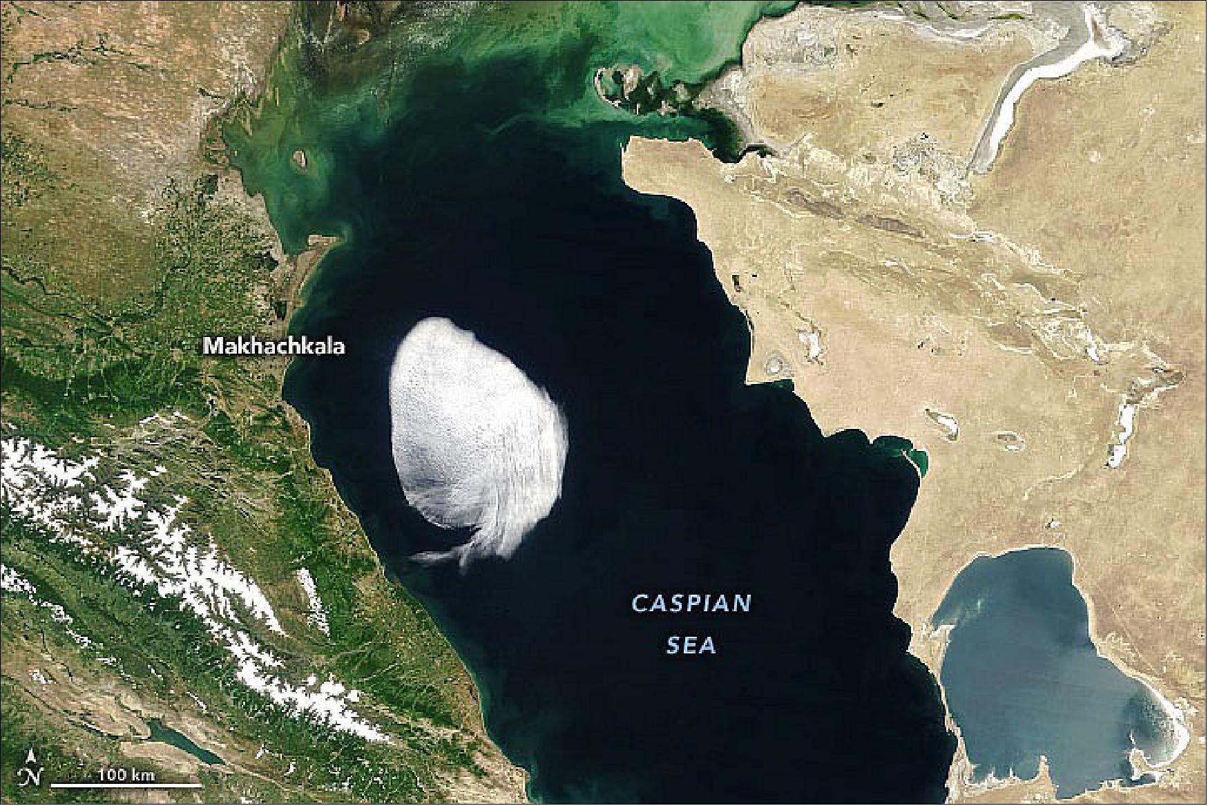
• June 16, 2022: On most days, clouds hover over at least part of the Caspian Sea, the planet’s largest inland body of water. But a cloud that drifted across the Caspian on May 28, 2022, looked more peculiar than most. 14) According to the SRON Netherlands Institute for Space Research, the cloud is a small stratocumulus. The cloud type is puffy like a cumulus cloud; cumulus is the Latin word for “heap” or “pile.” But unlike a cumulus cloud, the “heaps” in a stratocumulus cloud are clumped together, forming a widespread horizontal cloud layer. (Stratus is from a Latin verb that means “to spread out,” or “cover with a layer.”) The stratocumulus pictured here formed a layer spanning about 100 km (60 miles) across. Stratocumulus clouds form at low altitudes, generally between 600 and 2,000 meters (2,000 and 7,000 feet). This cloud was probably hovering at an altitude of about 1,500 meters (5,000 feet). In the late morning, the cloud was poised over the central Caspian. By the afternoon it had drifted toward the northwest and hugged the coast of Makhachkala, Russia, along a low-lying plain near the foothills of the Caucasus Mountains. It then drifted across the sea and dissipated when it reached land. The scenario also explains the cloud’s well-defined edges.
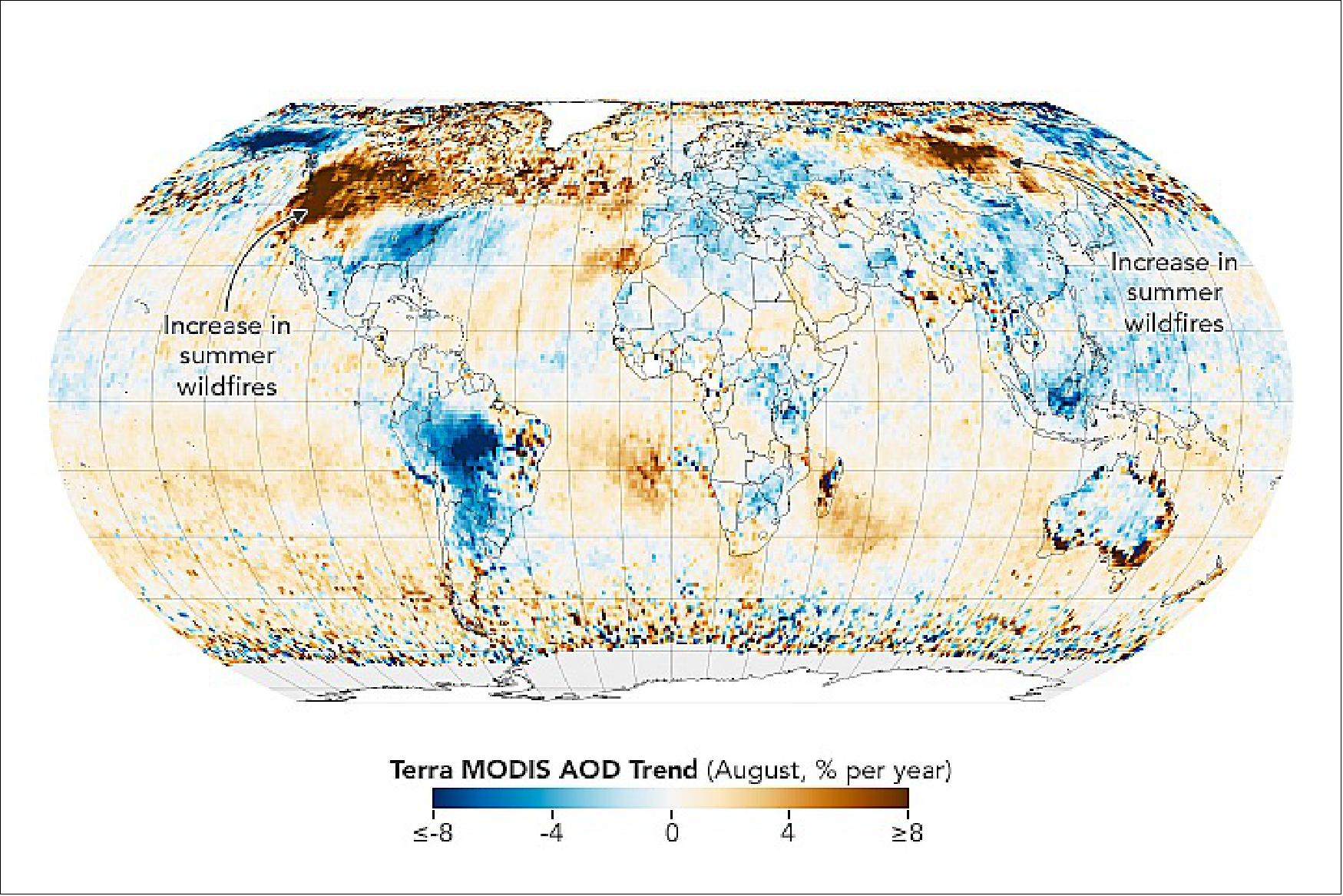
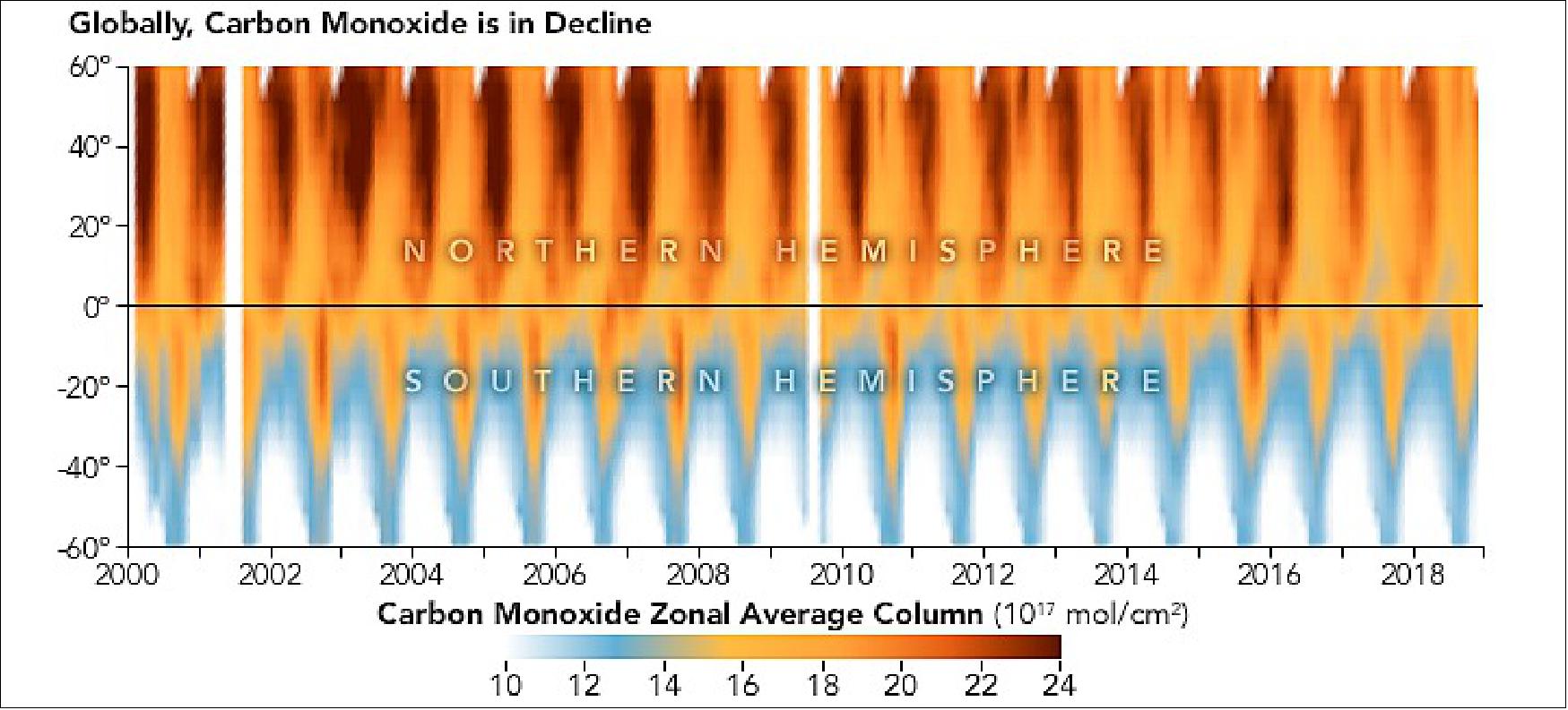
• May 27, 2022: NASA’s Terra satellite has been taking measurements of Earth’s atmosphere for more than two decades. One of the five sensors on board, Measurement of Pollution in the Troposphere (MOPITT), makes daily measurements of the air pollutant carbon monoxide. 15) Over the past two decades, MOPITT’s science team has observed a significant decline in global concentrations of carbon monoxide. Carbon monoxide also stays in the atmosphere for a few months, meaning it has plenty of time to mix and spread out. This makes it harder for researchers to pinpoint the sources or understand what factors are contributing to changes. But they do have ways of getting around this problem. By comparing MOPITT observations of carbon monoxide with measurements of shorter-lived pollutants that were released from some of the same sources better understanding of where the carbon monoxide came from and why the concentration of the gas had fallen was reported in Remote Sensing of Environment.
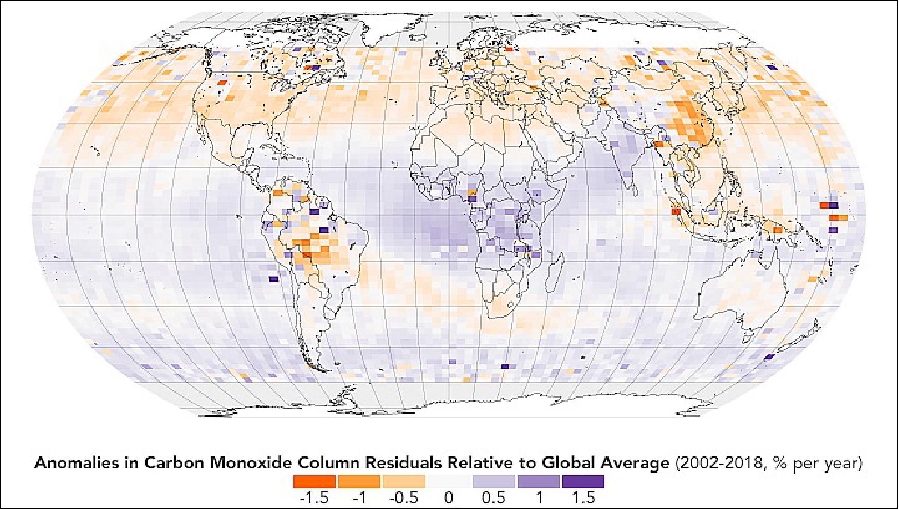
- In addition to analysing carbon monoxide and aerosol trends from MOPITT and MODIS, the researchers also considered observations from other satellite sensors and incorporated insights about regional aerosol emissions from a range of other research. In many places, there has been a trend toward using machinery rather than periodic burning to maintain land in rural areas. Parts of India, the U.S. Pacific Northwest, and the Caspian Sea region have experienced increases in aerosol particles for other reasons. In India, loose environmental controls, combined with growing populations and lots of agricultural burning, has likely fueled the increases in aerosols there. In the western U.S., the aerosol load has increased as drought and climate change have fueled more frequent and intense fires. The extra smoke has potentially exposed as many as 130 million people to toxic substances in recent years and threatens to reverse years of air quality gains. The data indicates a similar process may be playing out in Siberia—another region that has seen increased fire activity in recent years. Terra was launched in 1999 with an expected design life of six years.
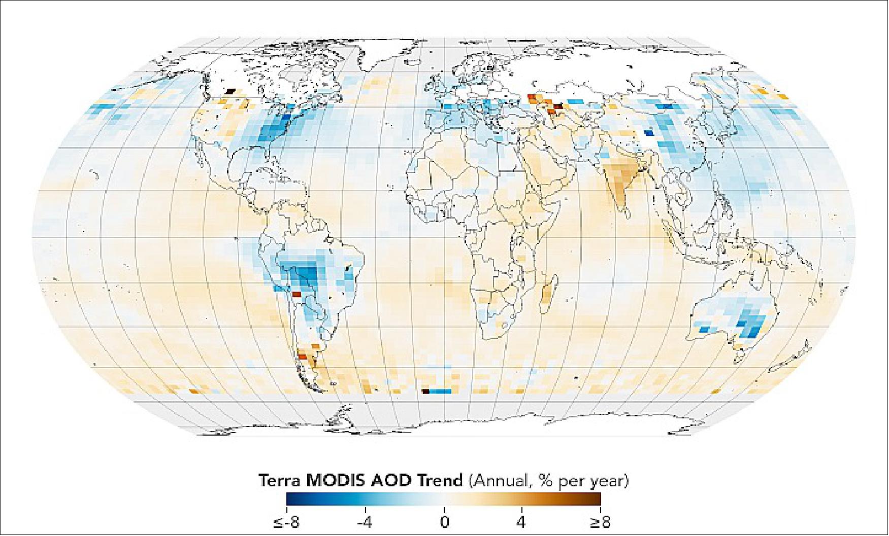
• May 26, 2022: For more than two decades, NASA’s Terra satellite has measured atmospheric concentrations of carbon monoxide (CO). The good news is that average levels of the toxic air pollutant have dropped by about 15 percent since 2000. However, the rate of decline has slowed, falling from about 1 percent per year in the earlier part of the record to about 0.5 percent per year in the later years. 16)Deciphering the reasons for declining carbon monoxide levels was complicated for Buchholz and colleagues because there are several sources of the pollutant. The seasonal peaks in the spring in both hemispheres are driven by changes in the availability of sunlight and hydroxyl radical (OH), a “detergent” molecule that removes carbon monoxide from the atmosphere by converting it into carbon dioxide. The reduction in light in winter reduces the amount of hydroxyl in the air, which allows levels of carbon monoxide to increase in the winter and early spring. Across the entire year, carbon monoxide levels are higher in the Northern Hemisphere, where there are more landmasses, people, and fires than in the Southern Hemisphere. (The white gaps in the top plot are time periods when there was no available data.). The seasonal spike in the Northern Hemisphere grows smaller and smaller toward the end of the record, a sign of cleaner skies and falling levels of the pollutant. In 2002-2003, extreme fire activity in western and southeastern Russia dramatically increased levels of carbon monoxide in the Northern Hemisphere. Biomass burning also declined in South America and likely contributed to the decline in carbon monoxide there. The changes over the ocean are likely the result of processes happening over the land before carbon monoxide was carried over the oceans by wind.
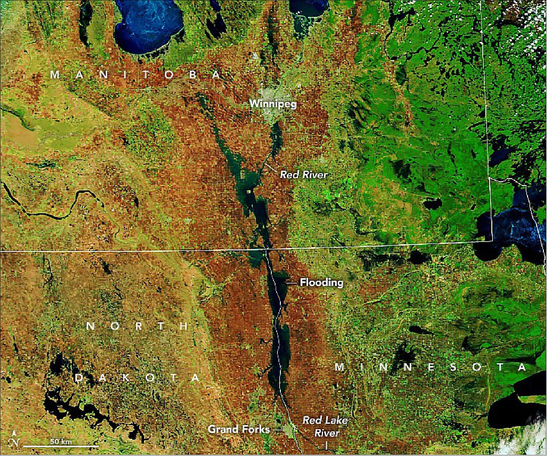
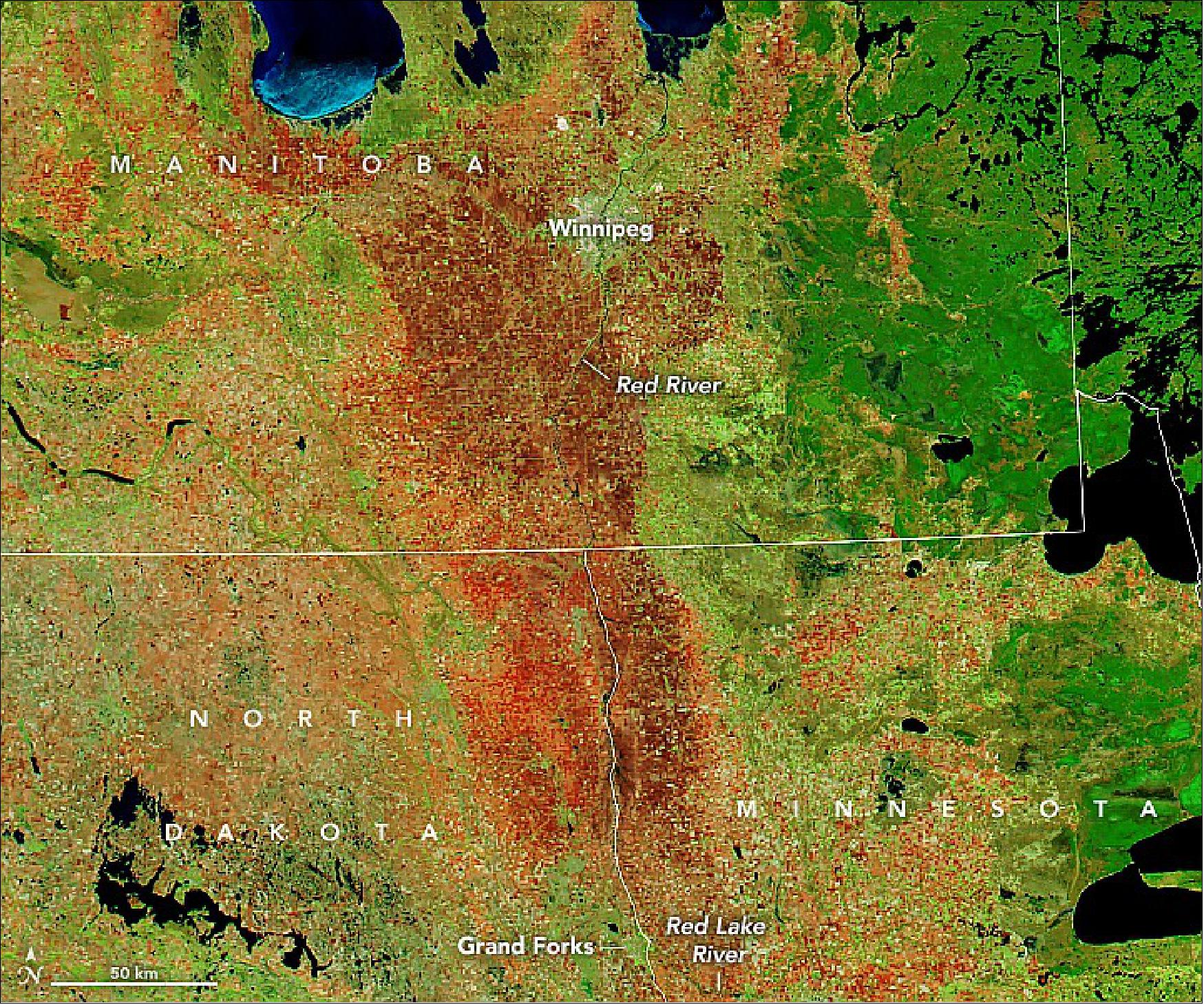
• May 12, 2022: The Red River Valley in Minnesota, North Dakota, and Manitoba is facing some of its worst flooding in a decade. An extreme spring blizzard, multiple rainstorms, and melting winter ice swelled the Red River of the North and its tributaries, driving them out of their banks and across a broad, flat floodplain. The deluge comes one year after the same region endured extreme drought. 18) According to the U.S. National Weather Service, the water level on the Red River at Pembina, North Dakota (near the U.S.–Canada border) crested at 52.27 feet (15.93 m) on May 8; The Red River remained in major flood stage at Oslo, Minnesota: river gauges measured 36.09 feet on May 11, while flood stage is 26 feet. According to Canadian authorities, the Red River flood this year is already the sixth largest on record (by volume) at Emerson, Manitoba. Forecasters were calling for more rain in the region on May 12. The flow and topography of the Red River basin are unusual, leading to somewhat regular spring flooding. This can lead the river to slow or back up onto the floodplain. The river valley is also nearly flat, and it runs through a trough that was shaped by continental glaciers about 10,000 years ago. The elevation drop along the river from Fargo, North Dakota to the Canadian border is roughly 130 feet (40 meters).
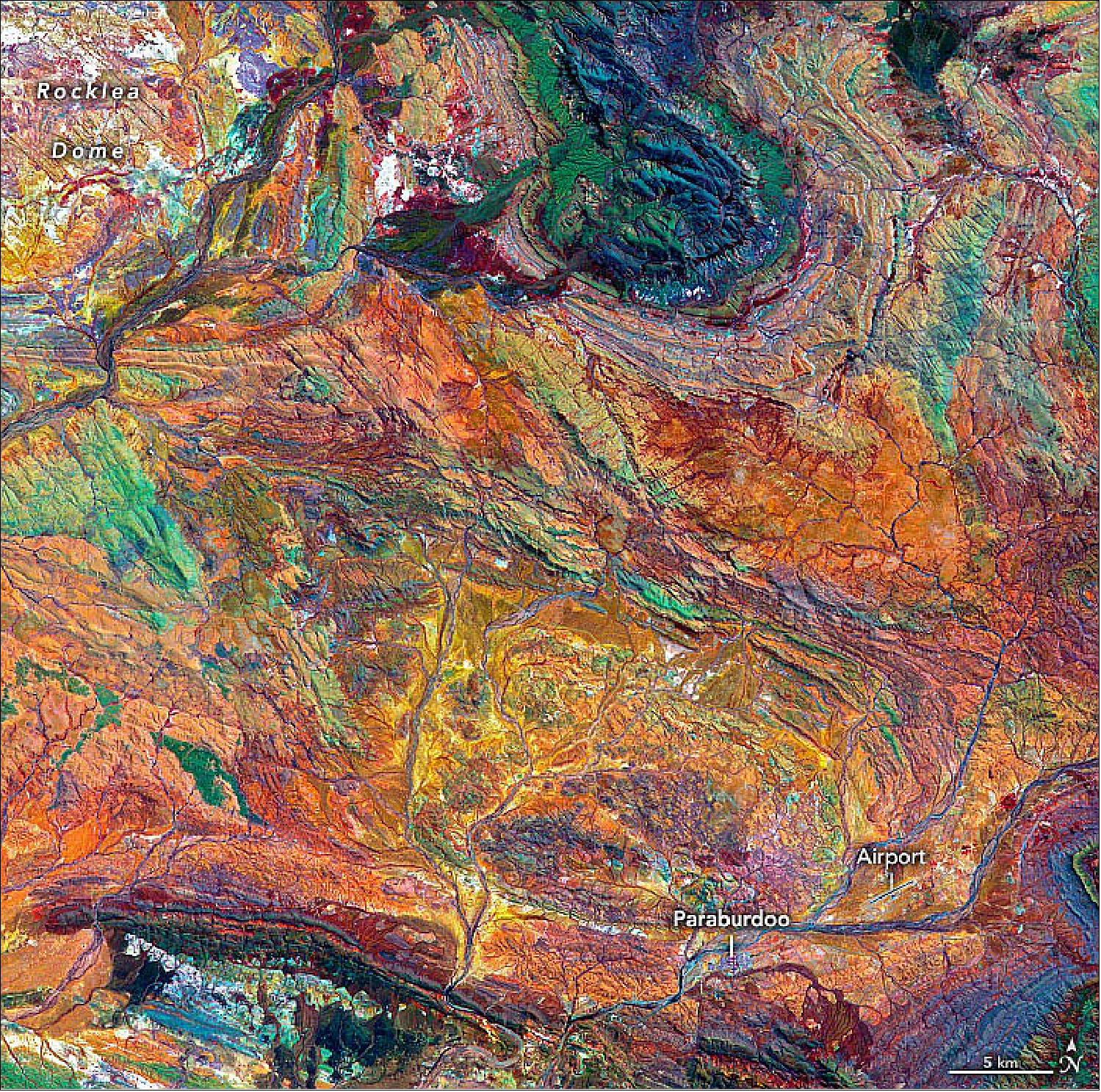
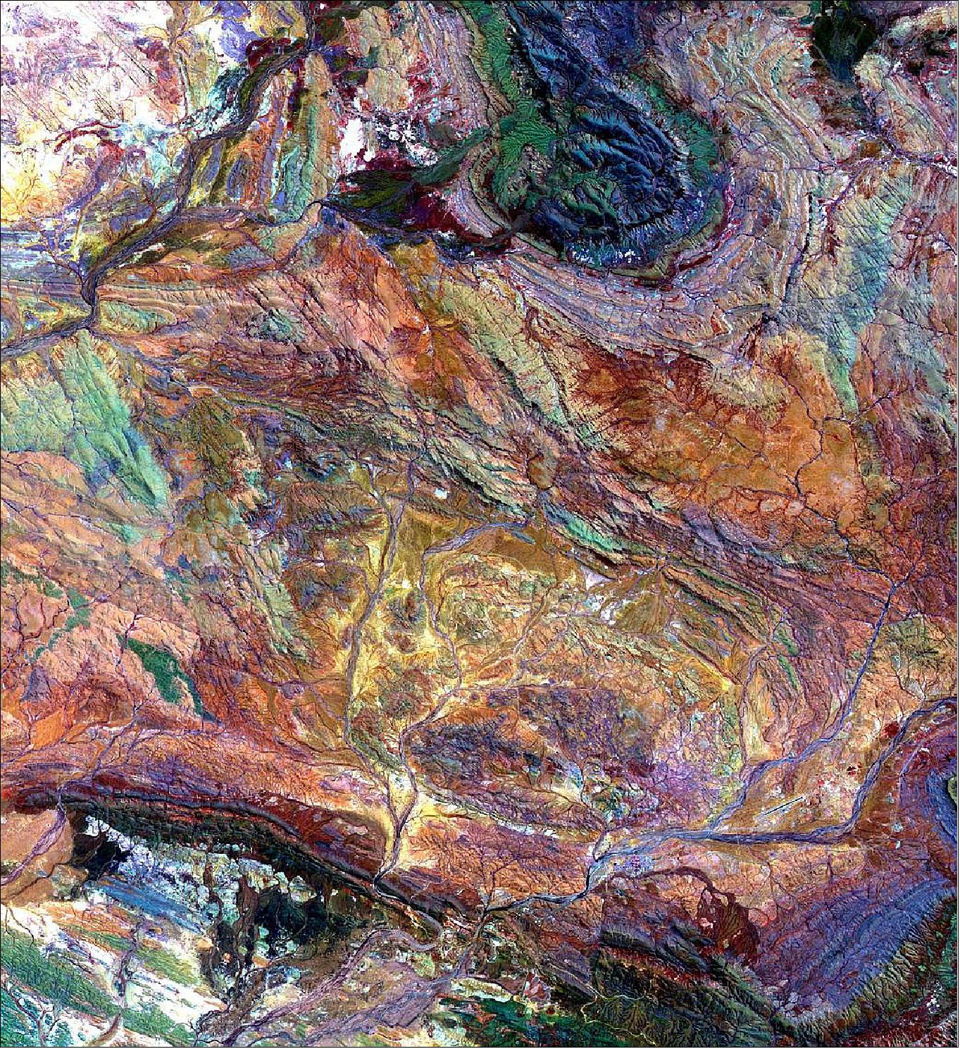
• April 4, 2022: Formed between 3.6 billion and 2.8 billion years ago, the rocks of the Pilbara Craton in Western Australia are some of the oldest on Earth. The iron-rich rocks here began forming before there was oxygen in Earth’s atmosphere or even life itself. The area also harbors evidence of some of the earliest life—3.45-billion-year-old fossil colonies of microbial cyanobacteria, the oldest known stromatolites on Earth. 19)The false-colour image shows part of the Hamersley Basin in Western Australia, which lies on the southern Pilbara Craton. A craton is the stable, geologically inactive core of an ancient continent. The Pilbara Craton has remained intact, surviving the affronts of plate tectonics and erosion since the Archean Eon (4 billion to 2.5 billion years ago). The imagery of the Pilbara Craton reveals billions of years of the rich geologic history of Western Australia.
- During the Archean, and the Proterozoic Eon that followed, multiple cratons assembled to form the Australian continent, leaving multiple basins and belts of buckled and folded rocks at their margins. The rocks of the basin preserve a record of the last ocean environment in the area before the cratons converged and closed the basin. Atop the granite and greenstone rocks of the Pilbara Craton lie the younger rocks of the Fortescue, Hamersley, and Turee groups, which were deposited between 2.7 billion and 2.3 billion years ago. Together these rocks form the Mount Bruce Supergroup, which holds a singular place in Australia’s geologic history. According to the Geological Survey of Western Australia, not only do these rocks hold the best-preserved sequence of Archean volcanic rocks, but they also include the most continuous rock record of the transition from the Archean to the Proterozoic 2.5 billion years ago (including a record of the Great Oxidation Event). These iron-rich rocks, including the world’s thickest and most extensive banded iron formations, form the basis of the iron-ore mining industry in the region. For example, in the top center of the image, the knob-shaped outcrop colored blue and green shows the rocks of the Hamersley Group—which includes four major banded-iron formations separated by sequences of iron-poor dolomites, shales, and volcanics. At the top left of the image, the white area shows the southeast portion of the Rocklea Dome, which is composed of light-colored granites.
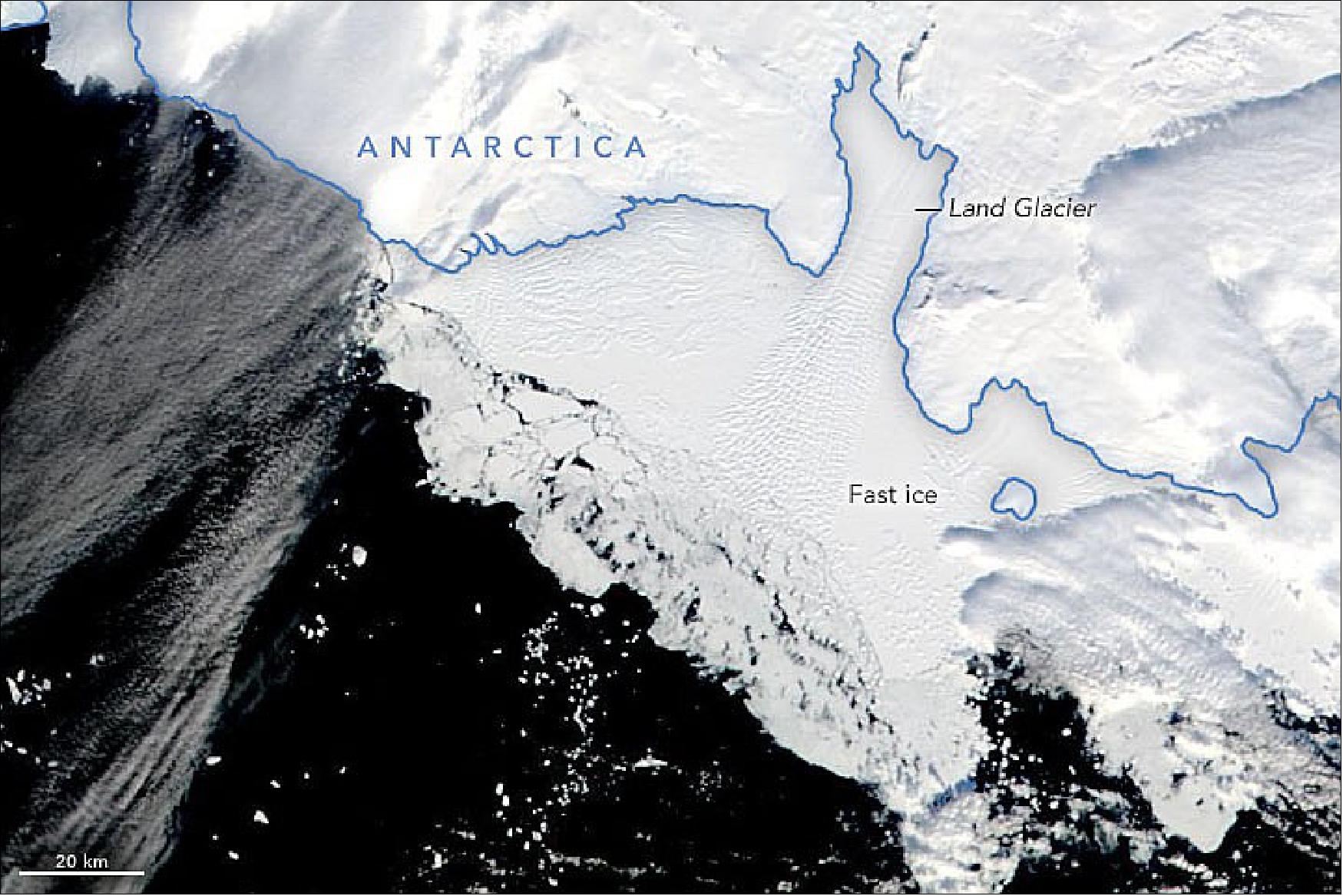
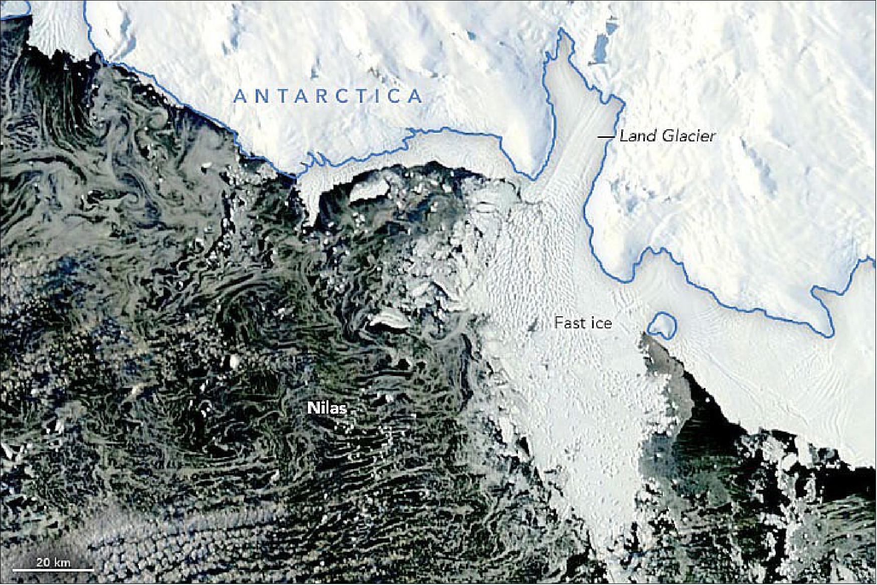
• April 2, 2022: Sea ice around Antarctica started to regrow after reaching the lowest extent ever observed in the satellite record in late February 2022. But on local scales, this transition from melting to freezing can display nuance. For example, near Land Glacier in West Antarctica, an area of old sea ice broke up as new ice formed in March. Around the same time, part of the glacier’s ice tongue crumbled away. 20) The February image displays a vast expanse of sea ice fastened to the edge of the coastline, and to the Land Glacier’s ice tongue and icebergs. Lowe explained that this “fast ice” often has a symbiotic relationship with glaciers and icebergs. Recent research using satellite observations showed that fast ice around parts of Antarctica, including off the coast of Marie Byrd Land, has been decreasing since MODIS records began around 2000. Still, a substantial patch remained at the time of the February image. By March, much of this old fast ice had broken apart. In the March image, the icebergs appear to be turning west into the direction of the remaining sea ice. The Coriolis effect will also influence the bergs’ flow, deflecting them toward the left of their path. Iceberg calving is a natural process for glaciers that terminate in the ocean. The glacier last lost a similar amount of floating ice during the austral winter of 2004. Another stage in the natural lifecycle of sea ice is visible in the March image: the growth of new sea ice.
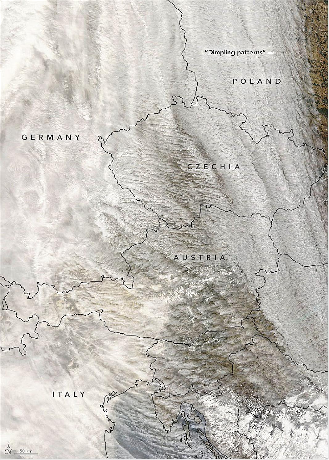
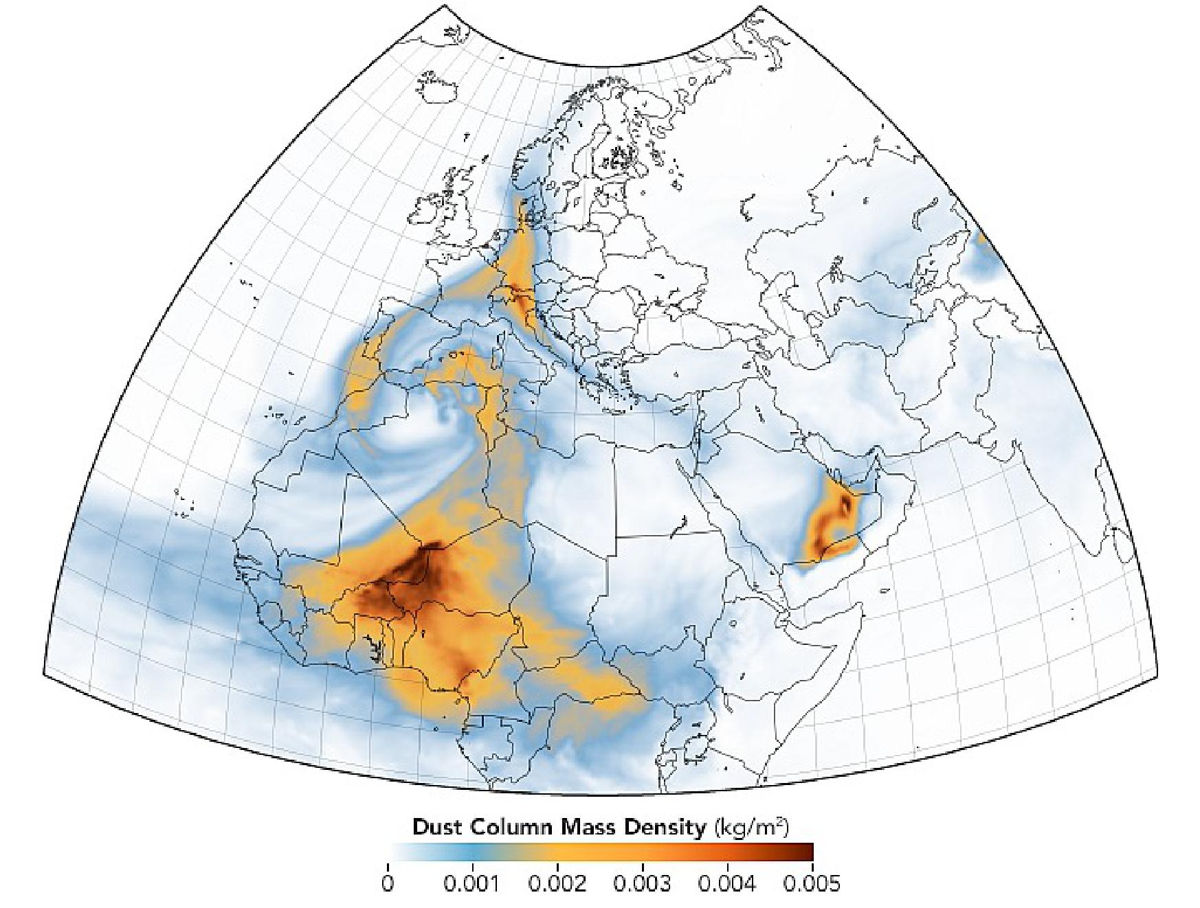
• March 31, 2022: In March 2022, several large storms carried clouds of Saharan dust to Europe. One of them also brought long-lasting, high-altitude cirrus clouds infused with dust, which led to extensive cloud cover—from Iberia to the Arctic—for more than a week. It was an unusual type of storm that scientists have only recently come to understand. Called a dust-infused baroclinic storm (DIBS), its hallmarks are icy clouds permeated with dust. 21) In mid-March, an atmospheric river of Saharan dust was entrained by a DIBS and lifted into the troposphere, reaching altitudes up to 10 km (6 miles). The dust acted as nucleation particles for ice, leading to the formation of icy high-altitude, dust-infused cirrus clouds. They persisted for nearly a week and covered large parts of Europe and Asia. The first storm started on March 15, 2022, over north central Europe and spread from Poland, Czechia, and Austria south to the eastern Mediterranean.
- On March 16, a second storm followed the classic pattern, spinning up closer to the source of the dust in Africa. The large, widespread dust cloud continued moving north over Europe toward Scandinavia and the Arctic Ocean. It then moved east over northern Russia before taking an anticyclonic turn and curving back down into Eastern Europe and the Black Sea region on March 20.
• March 9, 2022: The Pilbara in northwestern Australia exposes some of the oldest rocks on Earth, over 3.6 billion years old. The iron-rich rocks formed before the presence of atmospheric oxygen, and life itself. Found upon these rocks are 3.45 billion-year-old fossil stromatolites, colonies of microbial cyanobacteria. The image, acquired in October 2004, is a composite of ASTER bands 4-2-1 displayed in RGB. 22) With its 14 spectral bands from the visible to the thermal infrared wavelength region and its high spatial resolution of about 50 to 300 feet (15 to 90 meters), ASTER images Earth to map and monitor the changing surface of our planet and is one of five Earth-observing instruments launched Dec. 18, 1999, on the Terra satellite. The instrument was built by Japan's Ministry of Economy, Trade and Industry. A joint U.S./Japan science team is responsible for validation and calibration of the instrument and data products.
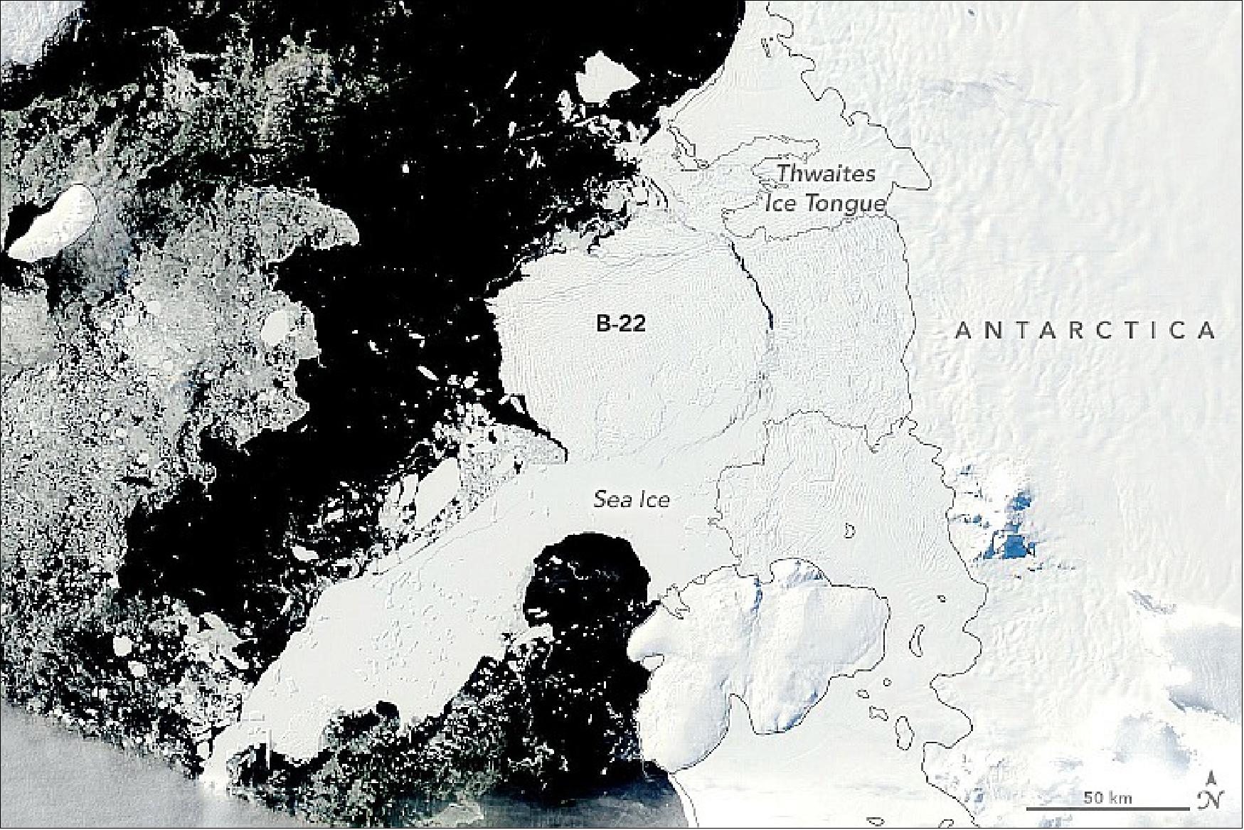
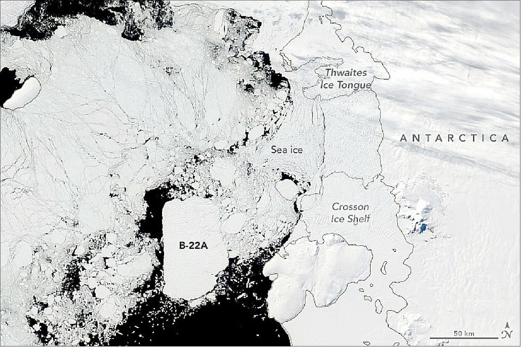
• March 1, 2022: The journey of every Antarctic iceberg is unique. Some drift many thousands of kilometers in the Southern Ocean before disintegrating and melting away. Others, like Iceberg B-22A, stay closer to home. In the span of 20 years, B-22A has strayed just 100 km (60 miles) from its birthplace, the floating ice tongue of Thwaites Glacier. 23) Studies have shown that the grounded iceberg plays an important role in stabilising sea ice in the area. In some years, a band of landfast sea ice has anchored to the iceberg and ice tongue. This landfast ice is thought to help buttress the Thwaites ice tongue and ice shelf, slowing the flow of ice toward the sea.
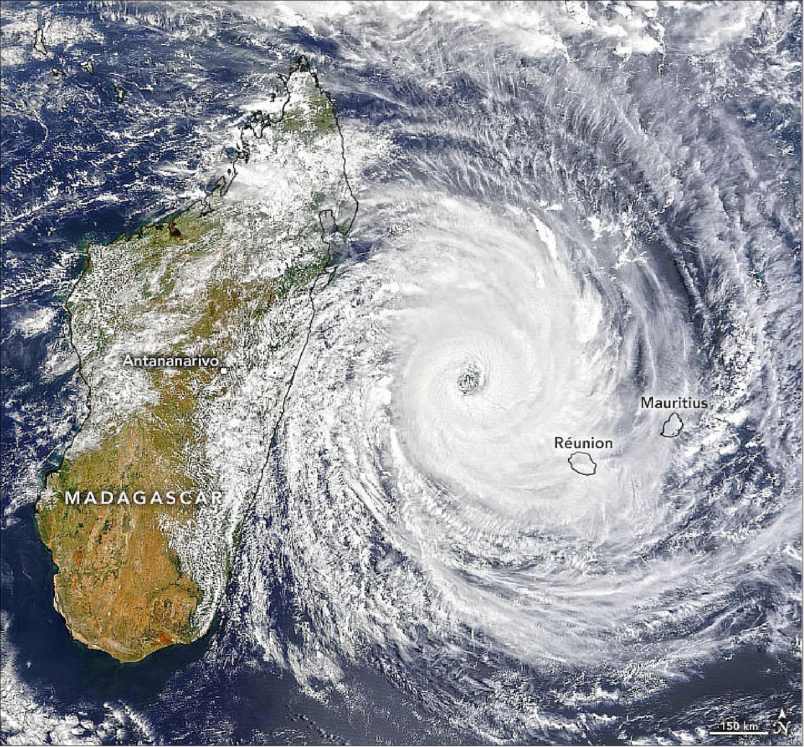
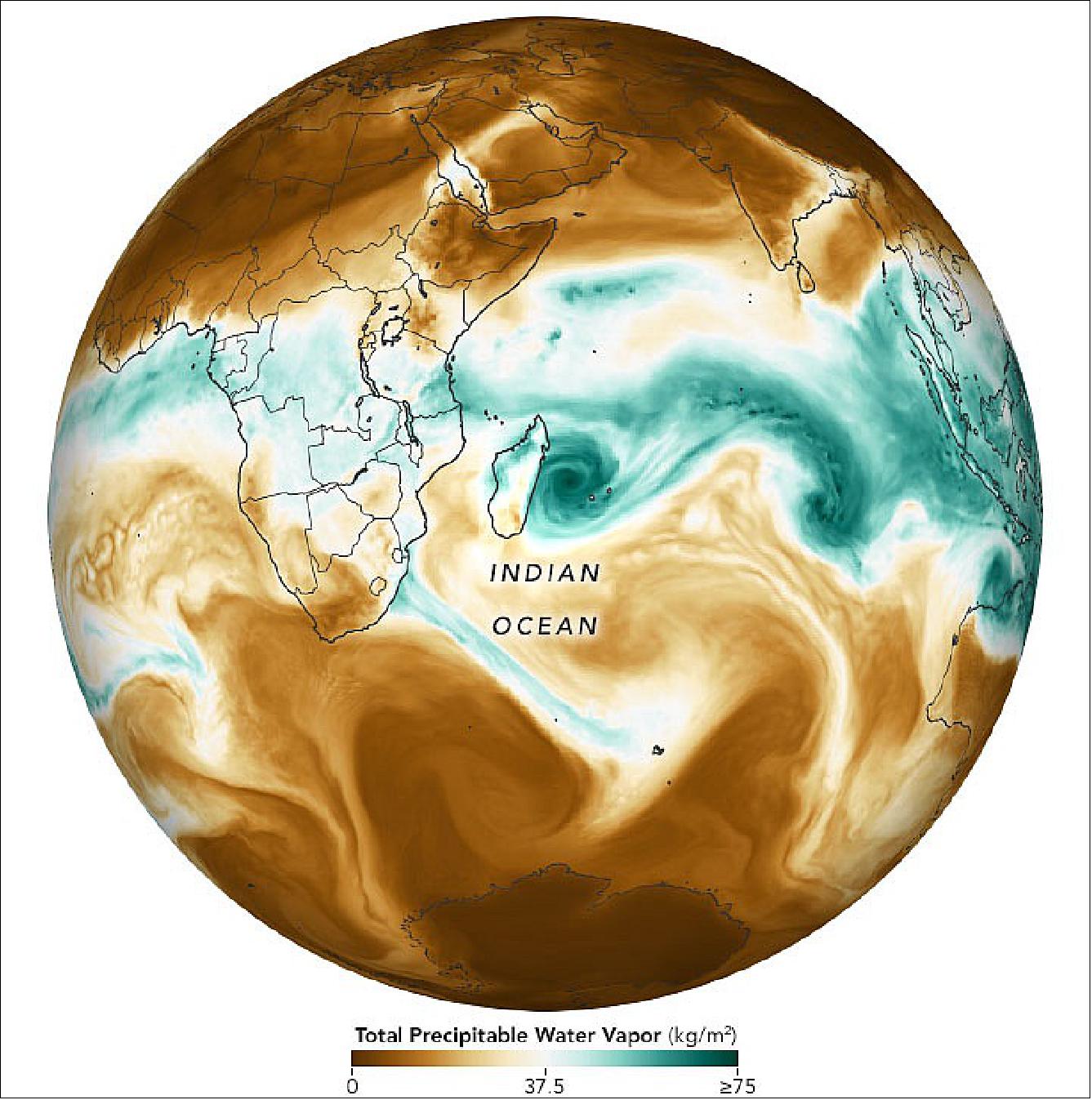
• February 5, 2022: After being soaked in mid-January 2022 by persistent, flooding rainstorms and Tropical Storm Ana, citizens of Madagascar are bracing for the arrival of another potent cyclone. Forecasters from the U.S. Joint Typhoon Warning Center suggest Cyclone Batsirai is likely to make landfall on February 5 in central Madagascar between Mahanoro and Mananjary as a category 2 storm. 24) The United Nations Office for the Coordination of Humanitarian Affairs estimated that 4.5 million people live within the projected path of the storm. Meteo Madagascar predicted 20 to 40 cm (8 to 16 inches) of rainfall and warned of the potential for widespread flooding in the east, southeast, and central highlands.
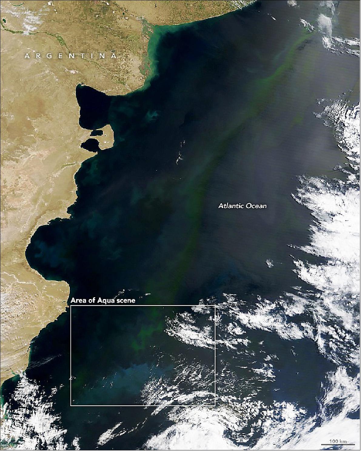
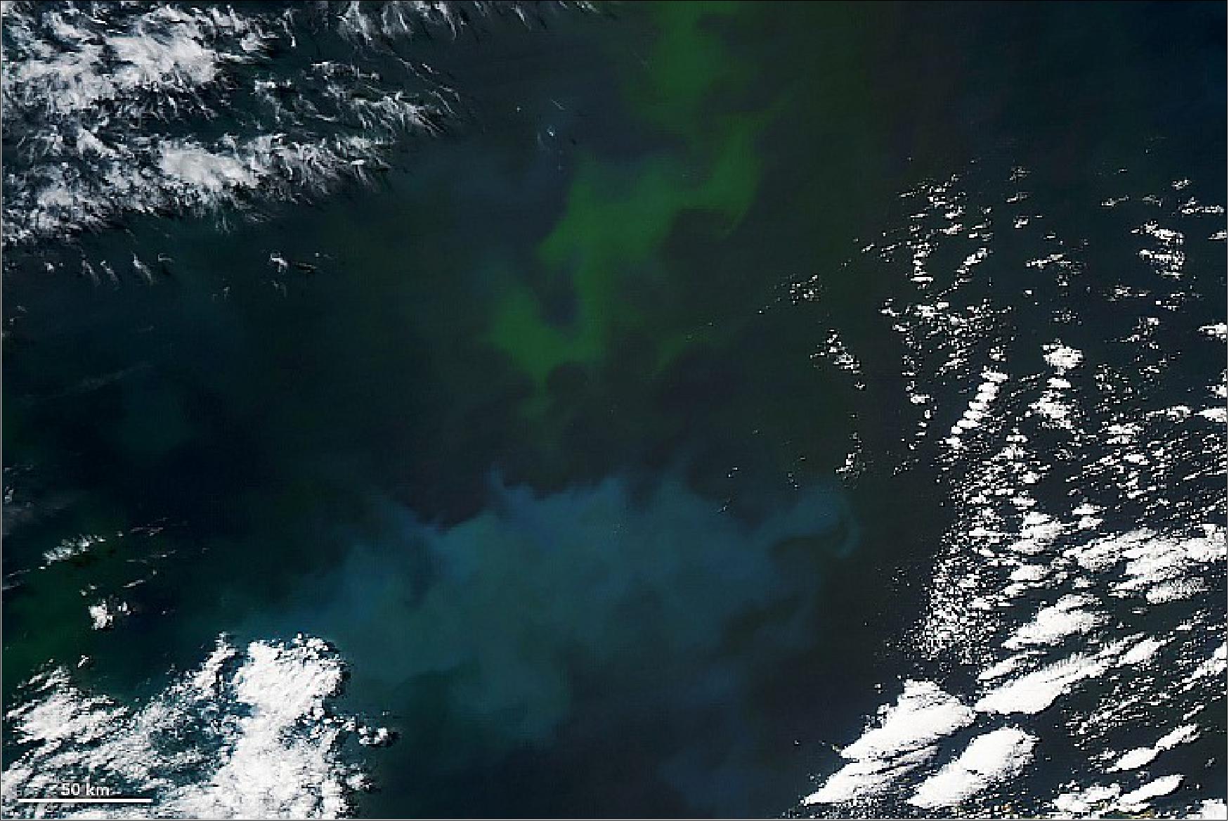
• January 28, 2022: Phytoplankton are sometimes called “the grass of the sea.” Like green plants on land, these floating, microscopic organisms play several key roles in making life on Earth possible. First, they are a source of food for zooplankton, shellfish, and marine creatures that eventually become food for other, larger creatures. They also produce a sizable amount of the oxygen in our oceans and atmosphere. And phytoplankton help remove carbon dioxide from Earth’s atmosphere, consuming it during photosynthesis and sinking it to the ocean depths in decaying cells and fecal matter from marine life (a phenomenon known as marine snow). 26)It is not possible to detect specific species from space, but the aquamarine stripes and swirls are likely coccolithophores—phytoplankton with microscopic calcite shells that give water a chalky colour. The various shades of green are probably diatoms, dinoflagellates, and related species. Imagers planned for future satellite missions should make it easier to identify types of phytoplankton from space. The patches of colour, in the images captured by MODIS, not only reveal the presence of phytoplankton, but also trace the edges of the dynamic eddies and currents that carry them. Off the coast of Argentina, Uruguay, and Brazil, warm currents from the tropics flow south and run into cooler currents flowing north from the Southern Ocean. They meet in a place known as the Brazil-Malvinas Confluence. At least seven different water masses of varying temperature, depth, and salinity arrive at this turbulent intersection, leading to vertical and horizontal mixing.
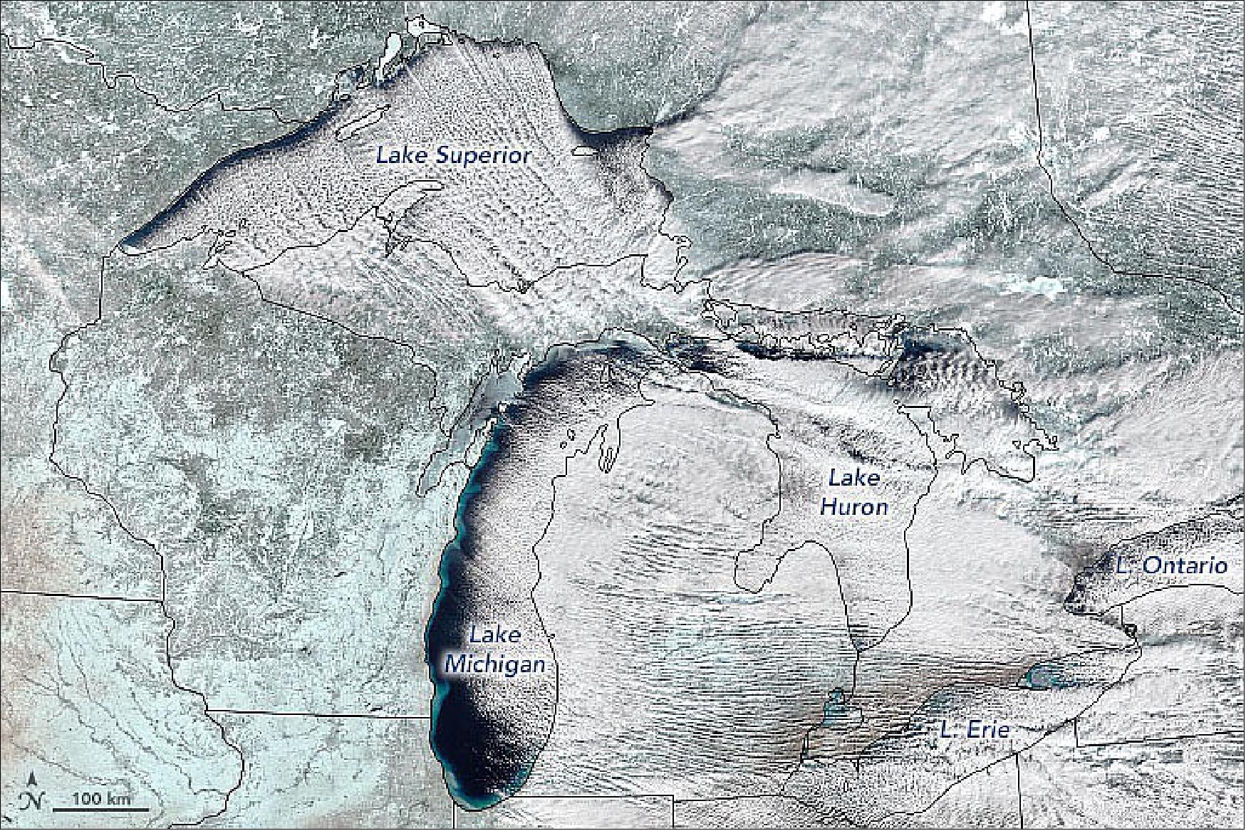
• January 17, 2022: Mid-winter in North America often brings blasts of cold wind blowing south from the Arctic or the Canadian interior. In addition to stirring up snowy weather and freezing the Great Lakes, the winds can create features that look like long white highways across the sky. 27) Cloud streets are parallel bands of cumulus clouds that form when frigid air near the surface blows over warmer waters, while a warmer air layer (a temperature inversion) rests over the top of both. The comparatively warm water gives up heat and moisture to the cold air, leading columns of heated air (thermals) to rise through the atmosphere. The warm air in the temperature inversion acts like a lid such that the moist, rising thermals hit the air mass above and roll over on themselves. This creates parallel horizontal cylinders of rotating air. On the upward side of the cylinders (rising air), the moisture cools and condenses into flat-bottomed, fluffy-topped cumulus clouds that line up parallel to the direction of the wind. Along the downward side (descending air), skies remain clear to make a cloudy-clear-cloudy striping pattern. Cloud streets are more common over the Great Lakes in the early part of winter, as the fresh water is still cooling down from summer and winter ice is starting to form. The cloud phenomenon also coincides sometimes with lake-effect snow downwind. In 2022 the MODIS instrument on NASA’s Terra satellite documented one such event.
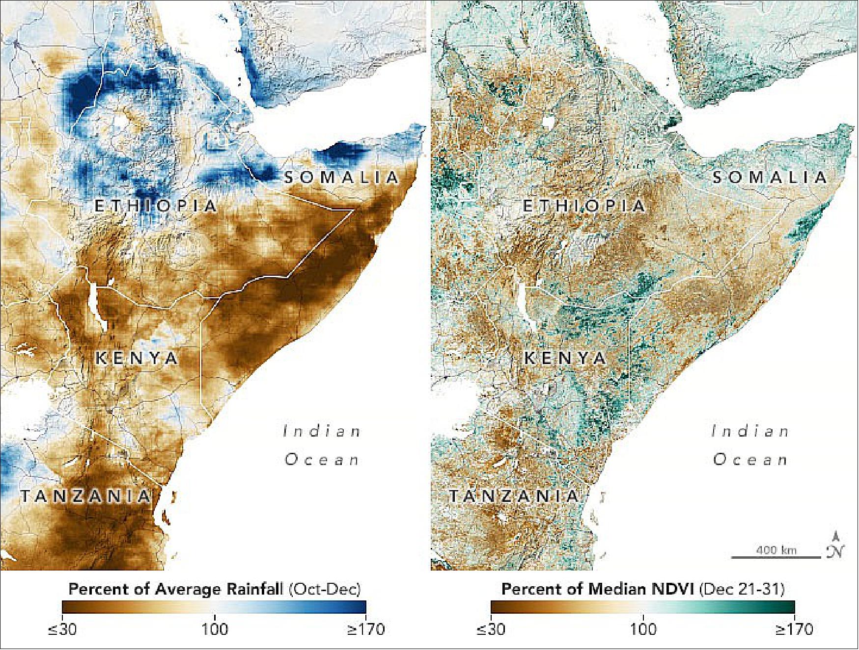
• January 7, 2022: Following three consecutive failed rainy seasons, more than 20 million people in eastern Africa now face some of the worst food security risks in 35 years. Climate and agriculture experts are advising governments and relief agencies to expect a significant need for food assistance in Somalia, Kenya, and Ethiopia. Climate change and ongoing La Niña conditions in the Pacific Ocean, half a world away, have contributed to the persistent dry weather and might bring more of it during the next rainy season. 28) The warnings come from the Famine Early Warning Systems Network (FEWS NET), a program supported by the U.S. Agency for International Development (USAID). FEWS NET assembles global and regional analyses of food security (particularly conditions for farming and livestock husbandry) to help governments and relief agencies plan for and respond to humanitarian crises. Several U.S agencies support FEWS NET; NASA provides satellite imagery and climate and weather data.
- Tropical countries within the Horn of Africa tend to have two rainy seasons: the gu in March, April, and May, and the deyr in October, November, and December. Similar conditions have also prevailed in southern and eastern Ethiopia. Successive rain shortfalls in eastern Africa have had a cumulative effect: smaller crop harvests; Production of cereals during the 2021 deyr was reduced by 50 to 70 percent, while maize and sorghum production were down 15 to 25 percent in 2020 and 50 percent in 2021. Current soil moisture forecasts from the NASA Hydrologic Analysis and Forecast System (NHyFAS) indicate there could be further reductions in soil moisture in the common months. The dire agricultural conditions have been exacerbated by the COVID-19 pandemic and by violent regional conflicts. And the region still has not fully recovered from the losses of a deep drought in 2016-17.
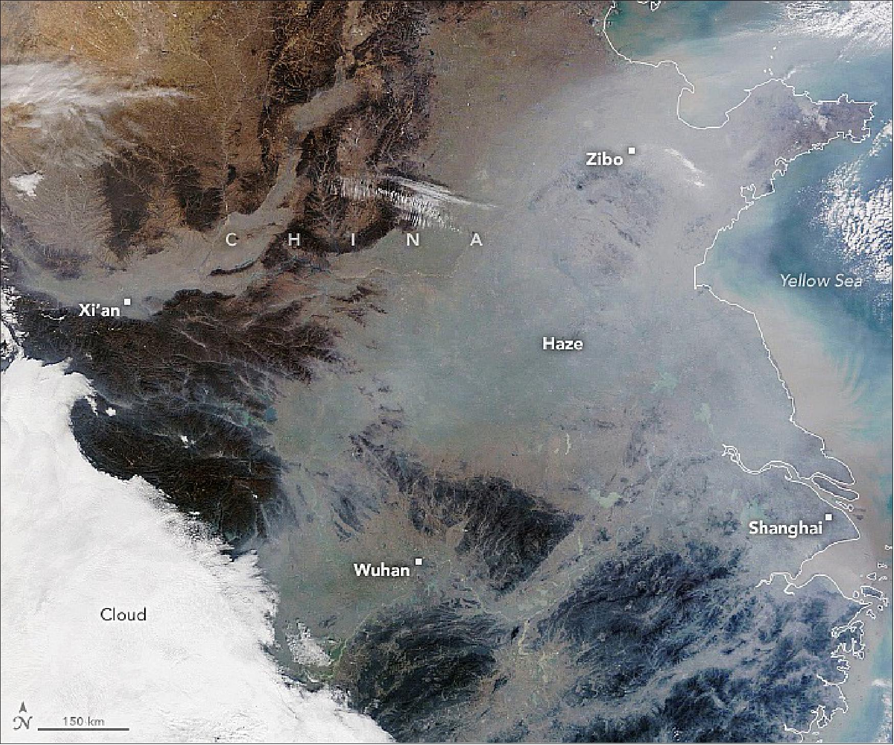
• January 6, 2022: The MODIS Instrument observed how despite levels of air pollution over China have decreased significantly in recent years, outbreaks of air pollution still regularly darken skies in some areas. 29) On the day that the image was acquired, several ground-based sensors in the region reported levels of fine particulate matter (PM2.5) in the very unhealthy and hazardous range, according to data published by The World Air Quality Project. That means PM2.5 levels were several times higher than the World Health Organization’s recommended limit of an average of 15 micrograms averaged over a day. Outbreaks of haze generally occur during winter because of temperature inversions. Air normally cools with altitude, but during an inversion warm air settles above a layer of cool air near the surface. The warm air acts like a lid and traps pollutants near the surface, especially in basins and valleys. Common sources of pollution in the winter include coal and wood burning for heat, industrial activity, and vehicle emissions. Smoke from fires and dust storms can also contribute to poor air quality. The region also recorded concerningly high nitrate levels.
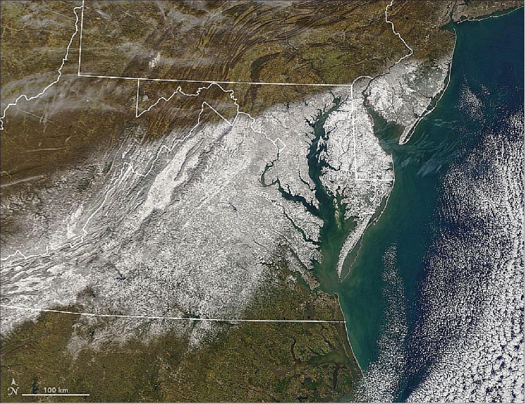
• January 4, 2022: After an unseasonably warm weekend in the eastern United States, a “Nor’easter” dumped a blanket of wet, heavy snow across the Mid-Atlantic region. 30) The storm blanketed the region with snow, closed schools, and snarled traffic.
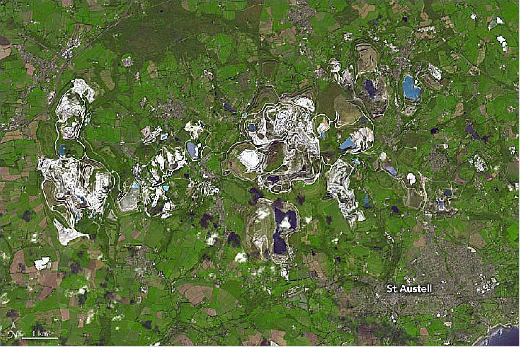
• January 03, 2022: The English porcelain industry began with the 1745 discovery of kaolinite, or “china clay,” at Tregonning Hill, Cornwall. By the early 19th century, the Cornish deposits were the largest known to the world. By 1910, Cornwall was producing 50 percent of the world’s china clay. The mines produced a million metric tons of clay each year, exporting 75 percent of it. Domestically, the clay was used to produce Wedgwood, Spode, and Minton china. 31) Clay mining left significant marks on the English landscape. Rain has since collected in many of the abandoned pits, forming ponds of various shades of blue (dependent on the amount of suspended clay minerals). Also, each ton of clay extracted from the ground resulted in multiple tons of waste products, which were piled in spoil tips. These pyramid-shaped mounds still dot the skyline and are sometimes called the Cornish Alps. Images of the area were obtained through the Advanced Spaceborne Thermal Emission and Reflection Radiometer (ASTER) aboard the Terra satellite on September 10, 2014.
Sensor Complement
Measurement Region | Measurement | Instruments used |
Atmosphere | Cloud properties | MODIS, MISR, ASTER |
Land surface | Land cover and land use change | MODIS, MISR, ASTER |
Ocean | Surface temperature | MODIS |
Cryosphere | Land ice change | ASTER |
ASTER (Advanced Spaceborne Thermal Emission and Reflection Radiometer)
ASTER is a Japanese instrument sponsored by METI (Ministry of Economy, Trade and Industry) and a cooperative project with NASA. The ASTER team leaders are Hiroji Tsu of ERSDAC (Japan) and Anne B. Kahle of JPL. ASTER management is provided by JAROS (Japan Resources Observation System Organization). ASTER was built by NEC, MELCO, Fujitsu, and Hitachi. A Joint US/Japan Science Team is responsible for instrument design, calibration, and validation. Previous instrument name: ITIR (Intermediate Thermal Infrared Radiometer).
Objective: Provision of high-resolution and multispectral imagery of the Earth's surface and clouds for a better understanding of the physical processes that affect climate change. Applications: studies of the surface energy balance (surface brightness temperature), plant evaporation, vegetation and soil characteristics, hydrologic cycle, volcanic processes, etc. 32) 33) 34) 35) 36) 37)
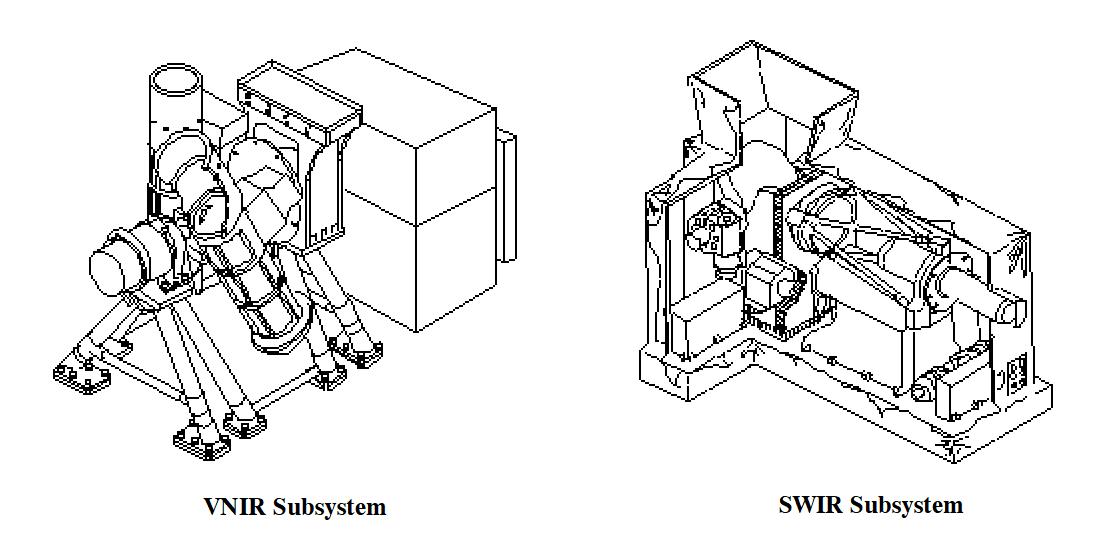
The ASTER instrument consists of three separate instrument subsystems; each subsystem operates in a different spectral region, has its own telescope(s), and is built by a different Japanese company. The subsystems are in the VNIR (Visible Near Infrared), SWIR (Shortwave Infrared) and TIR (Thermal Infrared) spectral regions. The VNIR and SWIR subsystems employ pushbroom imaging while the TIR subsystem performes whiskbroom imaging. ASTER is pointable in the cross-track direction such that any point on the globe may be observed at least once within 16 days in all 14 bands and once every 5 days in the VNIR bands. The absolute temperature accuracy is 3K in the 200-240 K range, 2K in the 240-270 K range, and 2 k in the 340-370 K range for TIR bands.
Total instrument mass=421 kg; power=463 W average, 646 W peak; data rate = 8.3 Mbit/s average and 89.2 Mbit/s peak; thermal control by 80 K Stirling cycle coolers, heaters, cold plate/capillary pumped loop, and radiators; pointing accuracy: for control = 1 km on ground (all axes), knowledge= 342 m on ground (per axis), stability=2 pixels for 60 seconds. shown in this figure.
Parameter | Band No | VNIR | Band No | SWIR | Band No | TIR |
Spectral bands in µm | 1 | 0.52 - 0.60 | 4 | 1.600 - 1.700 | 10 | 8.125 - 8.475 |
2 | 0.63 - 0.69 | 5 | 2.145 - 2.185 | 11 | 8.475 - 8.825 | |
3N | 0.76 - 0.86 | 6 | 2.185 - 2.225 | 12 | 8.925 - 9.275 | |
3B | 0.76 - 0.86 | 7 | 2.235 - 2.285 | 13 | 10.25 - 10.95 | |
Stereoscopic viewing | 8 | 2.295 - 2.365 | 14 | 10.95 - 11.65 | ||
9 | 2.360 - 2.430 |
|
| |||
Ground resolution | 15 m | 30 m | 90 m | |||
IFOV (nadir) | 21.5 µrad | 42.6 µrad | 128 µrad | |||
Data rate | 62 Mbit/s | 23 Mbit/s | 4.2 Mbit/s | |||
Cross-track pointing | ±24º (±318 km) | ±8.55º (116 km) | ±8.55º (116 km) | |||
Swath width | 60 km | 60 km | 60 km | |||
Detector type | Si (CCD of 5000 elements, | PtSi-Si Schottky barrier linear array, cooled to 80 K (Stirling cooler) | HgCdTe | |||
Data quantization | 8 bit | 8 bit | 12 bit | |||
Radiometric accuracy | 4% | 4% |
| |||
The cooling capacity of the SWIR cryocooler is a nominal value of 1.2 W at 70 K; the measured power consumption is 43.5 W, which satisfies the requirement that it be less than 55 W. The cooling capacity of the TIR cryocooler is a nominal value of 1.2 W at 70 K; the measured power consumption is 50 W, which satisfies the requirement that it be less than 55 W. 38)
The VNIR subsystem, built by NEC Corporation, is a reflecting-refracting improved Schmidt design. VNIR features two telescopes, one nadir-looking with a three-spectral-band detector, and the other backward-looking with a single-band detector. The backward-looking telescope provides a second view of the target area in band 3B for stereo observations. Cross-track pointing is accomplished by rotating the entire telescope assembly. Band separation is through a combination of dichroic elements and interference filters that allow all three bands to view the same ground area simultaneously. Calibration of the nadir-pointing detectors is performed with two halogen lamps.
| ASTER | TM on Landsat 4/5 | ||
Wavelength Region | Band No. | Spectral Range (µm) | Band No. | Spectral Range (µm) |
VNIR |
|
| 1 | 0.45 - 0.52 |
1 | 0.52 - 0.60 | 2 | 0.52 - 0.60 | |
SWIR | 4 5 | 1.60 - 1.70 2.145 - 2.185 | 5 | 1.55 - 1.75 |
7 | 2.08 - 2.35 | |||
TIR | 10 | 8.125 - 8.475 | 6 | 10.4 - 12.5 |
The SWIR subsystem, built by MELCO (Mitsubishi Electric Company), uses a nadir-pointing aspheric refracting telescope. Cross-track pointing is accomplished by a pointing mirror. The size of the detector/filter combination requires a wide spacing of the detectors, causing in turn a parallax error of about 0.5 pixels per 900 m of elevation. This error is correctable if elevation data (DEM) are available. Two halogen lamps are used for calibration. The maximum data rate is 23 Mbit/s. 39)
The TIR subsystem employs a Newtonian catadioptric system with aspheric primary mirror and lenses for aberration correction. The telescope of the TIR subsystem is fixed to the platform, pointing and scanning is done with a single mirror. The line of sight can be pointed anywhere in the range ± 8.54º in the cross-track direction of nadir, allowing coverage of any point on Earth over the platform's 16 day repeat cycle. Each channel uses 10 mercury cadmium telluride (HgCdTe) detectors in a staggered array with optical bandpass filters over each detector element to define the spectral response. Each detector has its own pre- and post-amplifier for a total of 50. The detectors are being operated at 80 K using a mechanical split-cycle Stirling cooler. - In scanning mode, the mirror oscillates at about 7 Hz with data collection occurring over half the cycle. The scanning mirror is capable of rotating 180º from the nadir position to view an internal full-aperture reference surface, which can be heated to 340 K. 40)
Overview of some ASTER instrument characteristics:
• The Visible Near InfraRed (VNIR) telescope subsystem features a backward viewing band (next to a nadir viewing band) for high-resolution along-track stereoscopic observation (two-line VNIR imager)
• Provision of multispectral thermal infrared data of high spatial resolution (8 to 12 µm window region, globally)
• ASTER provides the highest spatial resolution surface spectral reflectance, temperature, and emissivity data within the Terra instrument suite
• The instrument provides the capability to schedule on-demand data acquisition requests
• The VNIR and SWIR subsystems employ pushbroom imaging while the TIR subsystem performes whiskbroom imaging
• ASTER provides band-to-band registration of the 14 spectral bands, not only within each subsystem, but also among the three subsystems. Accuracies of 0.2 pixels within each subsystem and 0.3 pixels among different subsystems are achieved.
CERES (Clouds and the Earth's Radiant Energy System)
The CERES instrument of NASA/LaRC was built by Northrop Grumman (formerly TRW Space and Technology Group) of Redondo Beach, CA (PI: Bruce Wielicki). Objective: Long-term measurement of the Earth's radiation budget and atmospheric radiation from the top of the atmosphere to the surface; provision of an accurate and self-consistent cloud and radiation database (input to WCRP international programs like TOGA, WOCE, and GEWEX). Retrieval of cloud parameters in terms of measured areal coverage, altitude, liquid water content, and shortwave and longwave optical depths. Specific science objectives are: 41) 42) 43) 44)
• For climate change analysis, provide a continuation of the ERBE record of radiative fluxes at the top of the atmosphere (TOA), analyzed using the same algorithms that produced the ERBE data.
• Double the accuracy of estimates of radiative fluxes at TOA and the Earth's surface.
• Provide the first long-term global estimates of the radiative fluxes within the Earth's atmosphere.
• Provide cloud property estimates that are consistent with the radiative fluxes from surface to TOA.

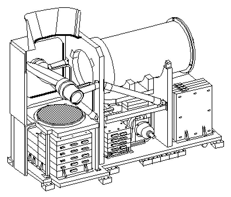
The CERES instrument assembly (of ERBE heritage) consists of a pair of broadband scanning radiometers (two identical instruments), referred to as FM-1 (Flight Module-1) and FM-2; one instrument operates in the cross-track mode for complete spatial coverage from limb to limb; the other one operates in a rotating scan plane (biaxial scanning) mode to provide angular sampling. The cross-track radiometer measurements are a continuation of the ERBS mission. The biaxially scanning radiometer provides angular flux information to improve model accuracy. A single cross-track CERES instrument is flown on TRMM (Tropical Rainfall Measuring Mission), while the dual-scanner instrument is flown on Terra (EOS/AM-1) and Aqua (EOS/PM-1).
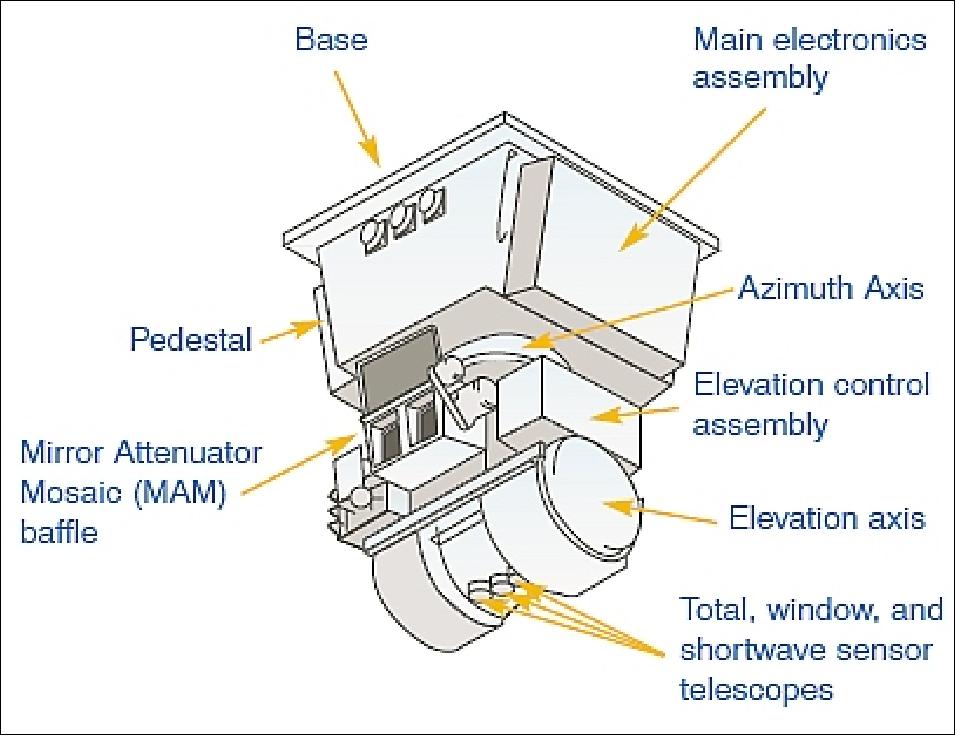
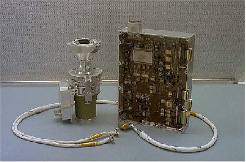
The CERES instrument consists of three major subassemblies: 1) Cassegrain telescope, 2) baffle for stray light, and 3) detector assembly, consisting of an active and compensating element. Radiation enters the unit through the baffle, passes through the telescope and is imaged onto the IR detector. Uncooled infrared detection is employed.
Instrument parameters (2 identical scanners): total mass of 100 kg , power = 103 W (average, 2 instruments), data rate = 20 kbit/s, duty cycle = 100%, thermal control by heaters and radiators, pointing knowledge = 180 arcsec. The design life is six years. CERES measures longwave (LW) and shortwave (SW) infrared radiation using thermistor bolometers to determine the Earth's radiation budget. There are three spectral channels in each radiometer:
- VNIR+SWIR: 0.3 - 5.0 µm (also referred to as SW channel); measurement of reflected sunlight to an accuracy of 1%.
- Atmospheric window: 8.0 - 12.0 µm (also referred to as LW channel); measurement of Earth-emitted radiation, this includes coverage of water vapor
-Total channel radiance in the spectral range of 0.35 - 125 µm;. reflected or emitted infrared radiation of the Earth-atmosphere system, measurement accuracy of 0.3%.
Limb-to-limb scanning with a nadir IFOV (Instantaneous Field of View) of 14 mrad, FOV = ±78º cross-track, 360º azimuth. Spatial resolution = 10-20 km at nadir. Each channel consists of a precision thermistor-bolometer detector located in a Cassegrain telescope.
Instrument calibration: CERES is a very precisely calibrated radiometer. The instrument is measuring emitted and reflected radiative energy from the surface of the Earth and the atmosphere. A variety of independent methods used to verify calibration: 45)
• Internal calibration sources (blackbody, lamps)
• MAM (Mirror Attenuator Mosaic) solar diffuser plate. MAM is used to define in-orbit shifts or drifts in the sensor responses. The shortwave and total sensors are calibrated using the solar radiances reflected from the MAM's. Each MAM consists of baffle-solar diffuser plate systems, which guide incoming solar radiances into the instrument FOV of the shortwave and total sensor units.
• 3-channel deep convective cloud test
- Use night-time 8-12 µm window to predict longwave radiation (LW): cloud < 205K
- Total - SW = LW vs Window predicted LW in daytime for same clouds <205K temperatures
• 3-channel day/night tropical ocean test
• Instrument calibration:
- Rotate scan plane to align scanning instruments TRMM, Terra during orbital crossings (Haeffelin: reached 0.1% LW, window, 0.5% SW 95% configuration in 6 weeks of orbital crossings of Terra and TRMM)
- FM-1 and FM-2 instruments on Terra at nadir
Instrument heritage | Earth Radiation Budget Experiment (ERBE) |
Prime contractor | Northrop Grumman (formerly TRW) |
NASA center responsible | LaRC (Langley Research Center) |
Three channels in each radiometer | Total radiance (0.3 to 100 µm); Shortwave (0.3 to 5 µm); Window (8 to 12 µm) |
Swath | Limb to limb |
Spatial resolution | 20 km at nadir |
Instrument mass, duty cycle | 50 kg/scanner, 100% |
Instrument power | 47 W (average) per scanner, 104 W (peak: biaxial mode) both scanners |
Data rate | 10 kbit/scanner |
Thermal control | Use of heaters and radiators |
Thermal operating range | 38±0.1ºC (detectors) |
FOV (Field of View) | ±78º cross-track, 360º azimuth |
IFOV | 14 mrad |
Instrument pointing requirements (3σ) |
|
Instrument size | 60 cm x 60 cm x 57.6 cm/unit |
The international CERES Science Team includes scientists from NASA, NOAA, US universities, France (CNRS), and Belgium (RMIB).
Data: A key element in the success of CERES, beyond the development of an instrument, is the development of data analysis and interpretation techniques for producing radiation and cloud products that meet the scientific objectives of the project.
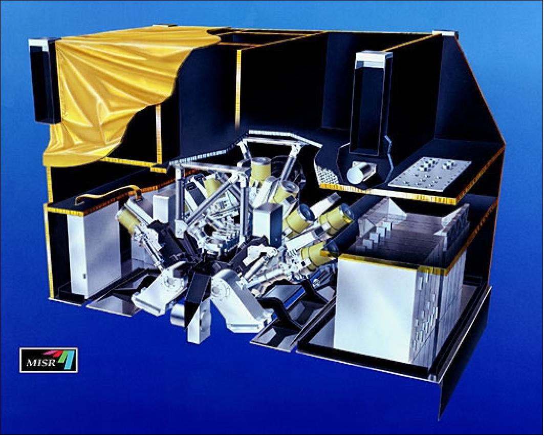
MISR (Multi-angle Imaging SpectroRadiometer)
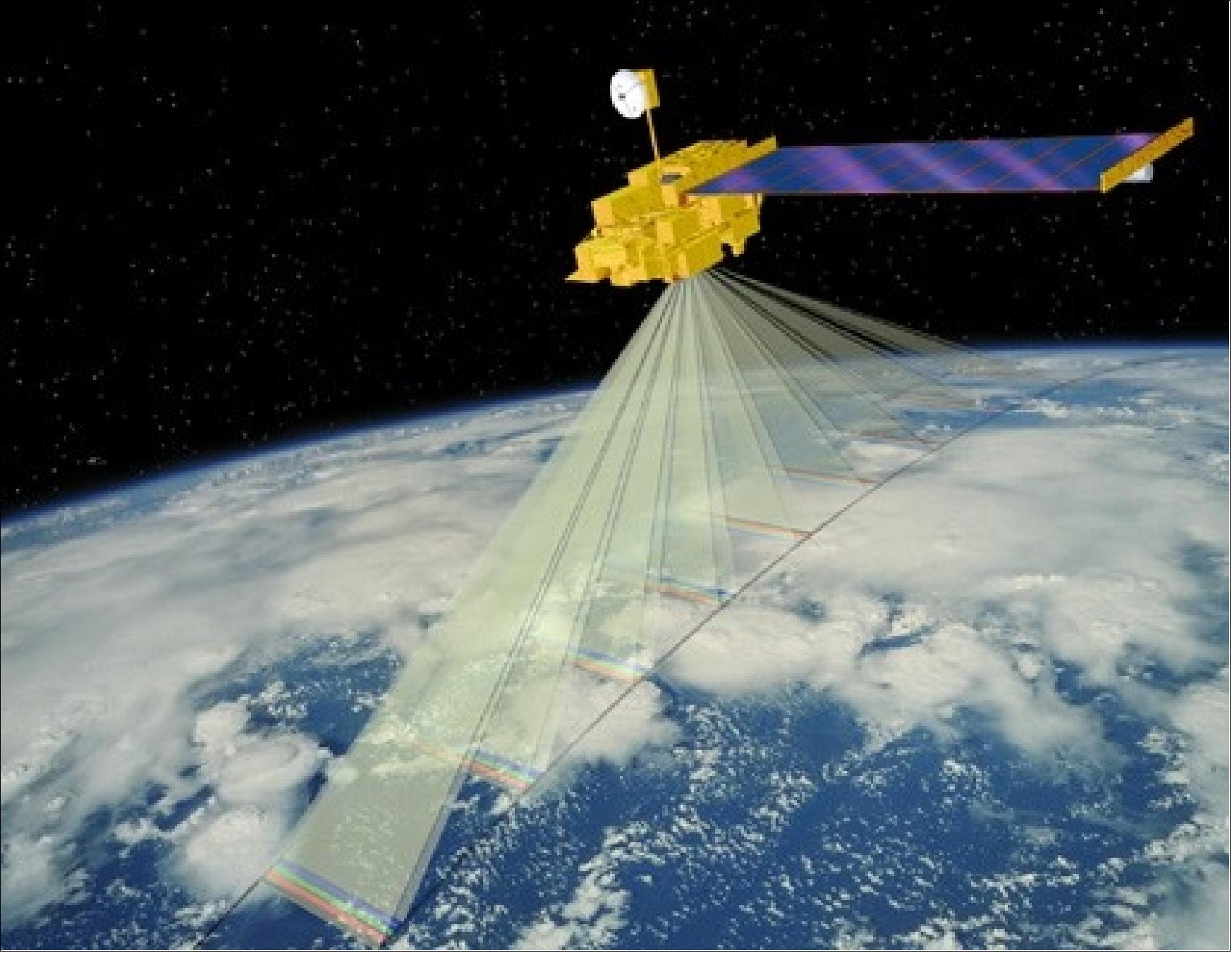
The MISR instrument was designed and developed by NASA/JPL (PI: D. J. Diner). Objective: provision of multiple-angle continuous sunlight coverage of the Earth with high spatial resolution (multidirectional observations of each scene within a time scale of minutes). MISR uses nine CCD pushbroom cameras to observe the Earth at nine discrete viewing angles: one at nadir, plus eight other symmetrical views at 26.1º, 45.6º, 60.0º, and 70.5º forward and aft of nadir. Images at each angle are obtained in four spectral bands centered at 0.446, 0.558, 0.672, and 0.866 µm. Each of the 36 instrument data channels (i.e. four spectral bands for each of the nine cameras) is individually commandable to provide ground sampling of 275 m, 550 m, or 1100 m. The swath is 360 km; multi-angle coverage (repeat cycle) of the entire Earth in nine days at the equator, and in two days at higher latitudes. By design, MISR is an along-track nine-line camera system, offering multidirectional observations of each ground (or target) scene. 46) 47) 48) 49)
Camera | View angle | Boresight angle | Swath offset angle | Effective focal length |
Df | 70.3º forward | 57.88º | -2.62º | 123.67 mm |
Cf | 60.2º forward | 51.30º | -2.22º | 95.34 mm |
Bf | 45.7º forward | 40.10º | -1.71º | 73.03 mm |
Af | 26.2º forward | 23.34º | -1.06º | 58.90 mm |
An | 0.1º nadir | -0.04º | 0.04º | 58.94 mm |
Aa | 26.2º aftward | -23.35º | 1.09º | 59.03 mm |
Ba | 45.7º aftward | -40.06º | 1.76º | 73.00 mm |
Ca | 60.2º aftward | -51.31º | 2.24º | 95.33 mm |
Da | 70.6º aftward | -58.03º | 2.69º | 123.66 mm |
Application: MISR provides global maps of planetary and surface albedo (brightness temperature), and aerosols and vegetation properties. Monitoring of global and regional trends in radiatively important optical properties (eg., opacity, single scattering albedo, and scattering phase function) of natural and anthropogenic aerosols.
MISR images are acquired in two observing modes: global and local. The global mode provides continuous planet-wide observations, with most channels operating at moderate resolution; some selected channels operate at the highest resolution for cloud screening and classification, image navigation, and stereo-photogrammetry. The local mode provides data at the highest resolution in all spectral bands and all cameras for selected 300 km x 300 km regions. In addition to data products providing radiometrically calibrated and geo-rectified images, global mode data will be used to generate two standard (level 2) science products: TOA (Top-of-Atmosphere)/Cloud Product and the Aerosol/Surface Product.
MISR on-orbit radiometric calibration is performed bi-monthly, using deployable white spectralon panels to reflect diffuse sunlight into the cameras, and a set of photodiodes to measure the reflected radiance. Additionally, vicarious calibrations using field and AirMISR data are done on six-month intervals. Geometric calibration of the cameras is done using ground control points.
Parameter | Description |
Mission life | 6 years |
Global coverage time | Every 9 days, with repeat coverage between 2-9 days depending on latitude |
Cross-track swath width | 360 km common overlap of all 9 cameras, FOV = ±60º along-track and ±15º cross-track. |
Nine CCD cameras | Named An, Af, Aa, Bf, Ba, Cf, Ca, Df, and Da where fore, nadir, and aft viewing cameras have names ending with letters f, n, a respectively and four camera designs are named A, B, C, D with increasing viewing angle respectively |
View angles at Earth surface | 0º, 26.1º, 45.6º, 60.0º, and 70.5º |
Spectral coverage | Four bands centered at 0.446, 0.558, 0.672, and 0.866 µm (blue, green, red, and NIR) |
Spatial resolution | 275 m, 550 m, or 1.1 km, selectable in-flight |
Detectors | CCDs, each camera with 4 independent line arrays (one per filter),1504 active pixels per line |
Radiometric accuracy | 3% at maximum signal |
Detector temperature | -5 ±0.1º C (cooled by thermo-electric cooler) of focal plane |
Structure temperature | 5º C |
Instrument mass, power | 148 kg, 131 W peak and 83 W average |
Instrument size | 0.9 m x 0.9 m x 1.3 m |
Data rate | 3.3 Mbit/s average, 9.0 Mbit/s peak |
MODIS (Moderate-Resolution Imaging Spectroradiometer)
MODIS is a NASA/GSFC instrument; prime contractor is Raytheon SBRS, Goleta, CA, formerly Hughes SBRS (Science team leader: V. Salomonson); MODIS algorithm development by an international team of scientists from USA, UK, Australia, and France; there are four discipline groups: Atmosphere, Land, Oceans, and Calibration. 50) 51) 52) 53)
The instrument is flown on the Terra and Aqua satellites (prime instrument). Objective: to measure biological and physical processes on a global basis on time scales of 1 to 2 days. Specific science goals are:
• To determine surface temperature at 1 km resolution, day and night, with an absolute accuracy of 0.2 K for ocean and 1 K for land
• To obtain ocean color (ocean-leaving spectral radiance) from 415 to 653 nm
• To determine chlorophyll fluorescence within 50% at surface water concentrations of 0.5 mg per cubic meter of chlorophyll a
• To obtain chlorophyll a concentrations within 35%
• To obtain information on vegetation and land surface properties, land cover type, vegetation indices, and snow cover and snow reflectance
• To obtain cloud cover with 500 m resolution by day and 1000 m resolution at night
• To obtain cloud properties and aerosol properties
• To determine information on biomass burning
• To obtain global distribution of atmospheric stability and total precipitable water.

Parameter | Value | Parameter | Value |
Instrument type | Opto-mechanical design (whiskbroom scanner) | Data rate | 10.6 Mbit/s (peak daytime), 6.1 Mbit/s (orbital average) |
Scan rate | 20.3 rpm | Data quantization | 12 bit |
Telescope | 17.8 cm diameter off-axis, afocal (collimated) with intermediate field stop | Spatial resolution | 250 m (bands 1-2) |
Size | 1.0 m x 1.6 m x 1.0 m | Swath width, FOV | 2330 km, 110º (1354 pixels in cross-track) |
Mass | 229 kg | Swath length/scan | 10 km (10 pixels in parallel along track) |
Power | 162.5 W | Design life | 6 years |
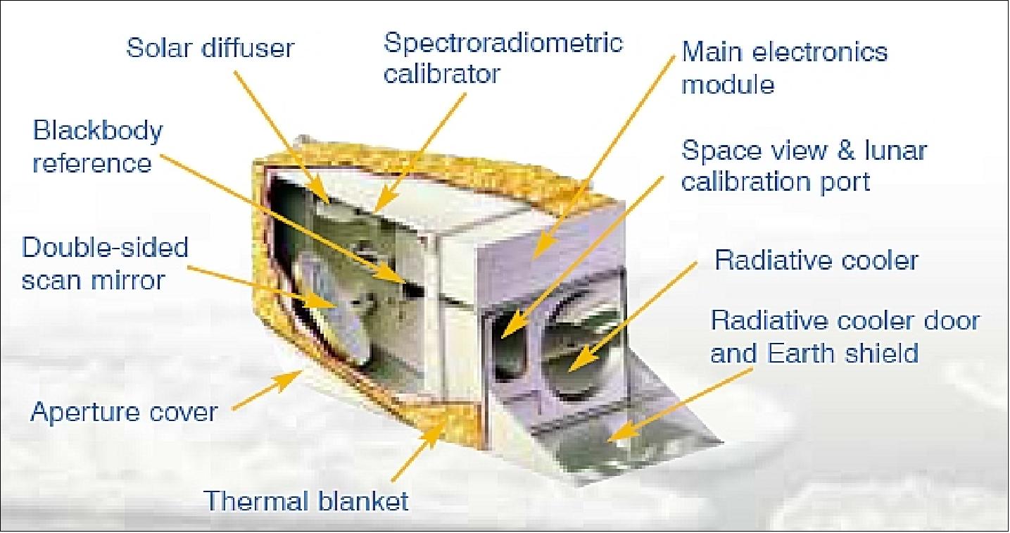
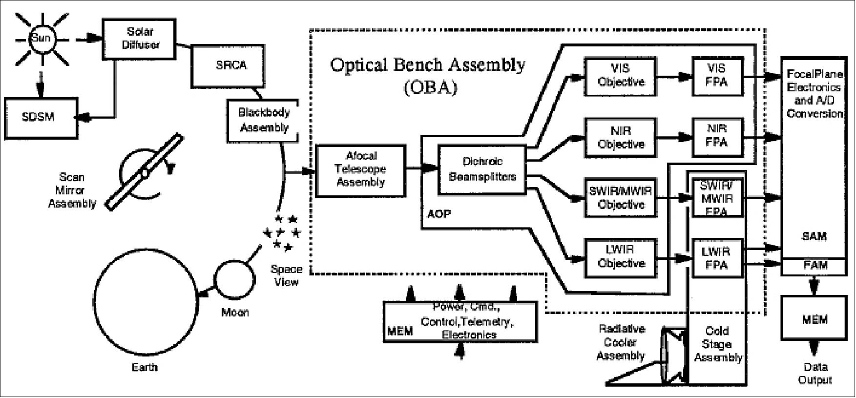
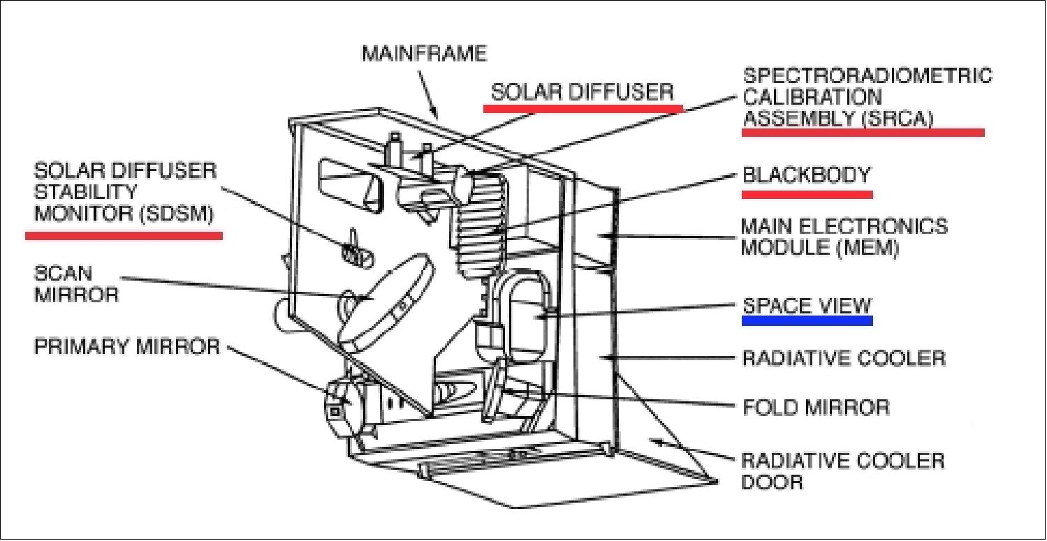
MODIS is an optomechanical imaging spectroradiometer (whiskbroom type), consisting of a cross-track scan mirror (continuously rotating double-sided scan mirror assembly) and collecting optics, and a set of linear detector arrays with spectral interference filters located in four focal planes. To accommodate frequent infrared calibration (every 1.47 s), a 360º rotating paddle-mirror is centered within a scan cavity to provide the optical subsystem with sequential views of the five calibrators and the Earth.
The optical arrangement provides imagery in 36 discrete bands between 0.4 and 14.5 µm (21 bands within 0.4-3.0 µm range, 15 bands within 3-14.5 µm range). The spectral bands provide a spatial resolution of 250 m, 500 m, and at 1 km at nadir. MODIS heritage: AVHRR (POES), HIRS (POES), TM (Landsat), CZCS (Nimbus-7). In fact, the MODIS instrument is considered to be a next-generation AVHRR instrument, having 36 bands (AVHRR/3 has 6) and a spatial resolution of 250 m (AVHRR has 1 km).
A high-performance passive radiative cooler provides cooling to 83 K for the infrared bands on two HgCdTe FPAs (Focal Plane Assemblies). A new photodiode-silicon readout technology for the VNIR range provides unsurpassed quantum efficiency and low-noise readout with a very good dynamic range.
MODIS polarization sensitivity < 2% for the visible range out to 2.2 µm; the performance goal for SNR (Signal-to-Noise Ratio) and NEΔT (Noise-Equivalent Temperature Difference) values is 30-40% better than the required values in Table 9.; absolute irradiance accuracy of 5% for <3 µm and 1% for >3 µm; absolute temperature accuracy of 0.2 K for oceans and 1 K for land; daylight reflection and day/night emission spectral imaging; swath width of 2330 km at 110º FOV; scan rate = 20.3 rpm across track; instrument mass = 250 kg; duty cycle = 100%; power = 225 W (average); data rate = 6.2 Mbit/s (average), 10.6 Mbit/s (peak daytime), 3.2 Mbit/s (night); quantization = 12 bit. Instrument IFOV (spatial resolution) = 250 m (bands 1-2), =500 m (bands 3-7), = 1000 m (bands 8-36).
The observations are made at three spatial resolutions (nadir): 0.25 km for bands 1-2 with 40 detectors per band, 0.5 km for bands 3-7 with 20 detectors per band, and 1 km for bands 8-36 with 10 detectors per band. All the detectors, aligned in the along-track direction, are distributed on four focal plane assemblies (FPAs) according to their wavelengths: visible (VIS), near infrared (NIR), short- and mid-wave infrared (SMIR), and long-wave infrared (LWIR).
Primary Use | Band No. | Bandwidth | Spectral Radiance | Required SNR | Spatial |
Land/Cloud | 1 | 0.620 - 0.670 | 21.8 | 128 | 250 m |
Land/Cloud | 3 | 0.459 - 0.479 | 35.3 | 243 | 500 m |
Ocean Color/ | 8 | 0.405 - 0.420 | 44.9 | 880 | 1000 m |
Atmospheric | 17 | 0.890 - 0.920 | 10.0 | 167 | |
Surface/Cloud | 20 | 3.660 - 3.840 | 0.45 | (0.05) | |
Atmospheric | 24 | 4.433 - 4.598 | 0.17 | (0.25) | |
Cirrus Clouds | 26 | 1.360 - 1.390 | 6.00 | 150 | |
Water Vapor | 27 | 6.535 - 6.895 | 1.16 | (0.25) | |
Ozone | 30 | 9.580 - 9.880 | 3.69 | (0.25) | |
Surface/Cloud | 31 | 10.780 - 11.280 | 9.55 | (0.05) | |
Cloud Top | 33 | 13.185 - 13.485 | 4.52 | (0.25) |
MODIS onboard calibration employs various techniques for comprehensive verification of spectral, radiometric and spatial measurements. They include: 54) 55) 56) 57)
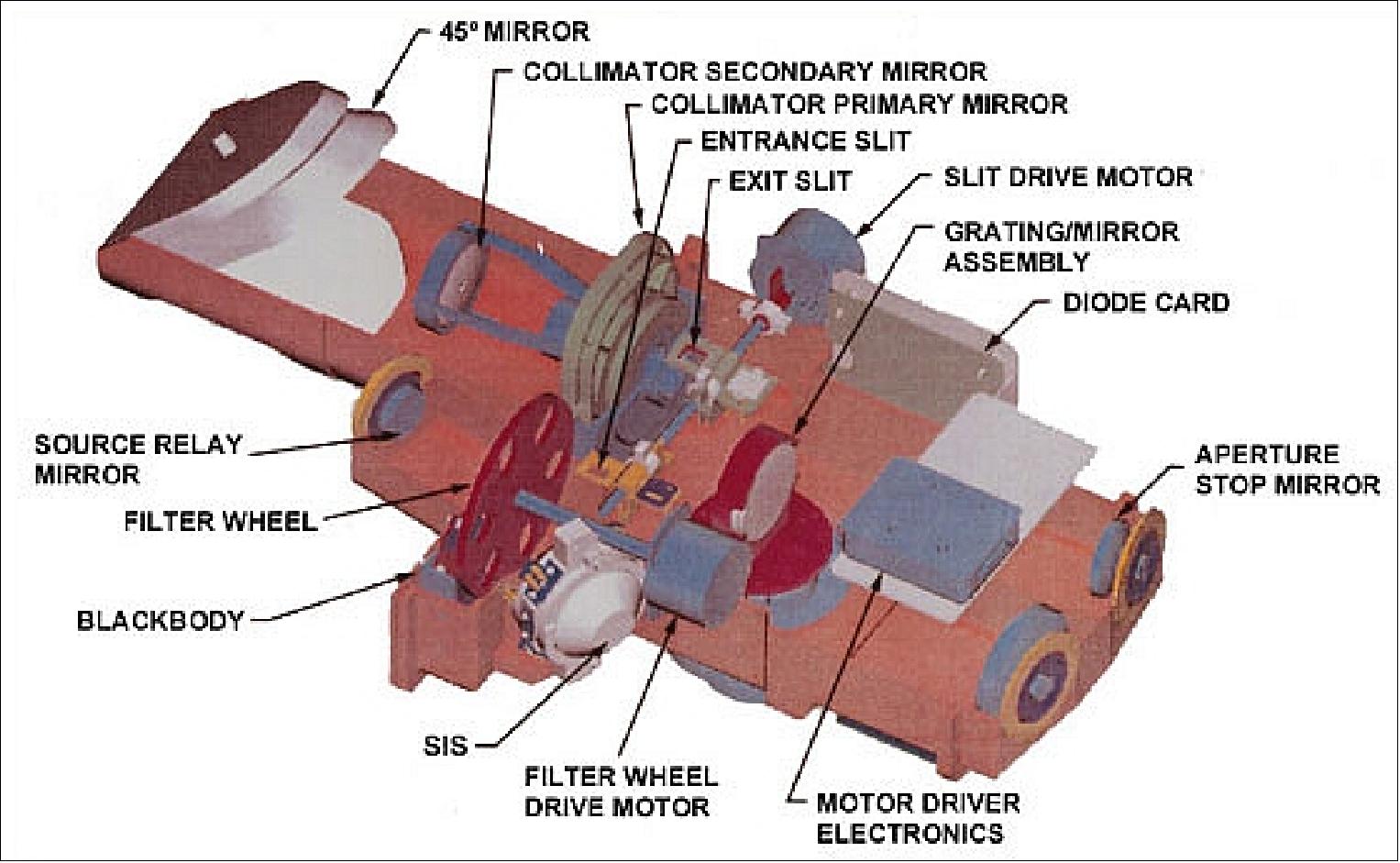
• Spectroradiometric Calibration Assembly (SRCA)
- Spectral calibration of reflective channel channel bandpasses
- Verification of spectral band registration
- DC restoration on every scan using a direct view of space
- Lunar calibration via the space-view port as well as periodic rotations of the S/C to enable full scans across the moon through the active scan aperture
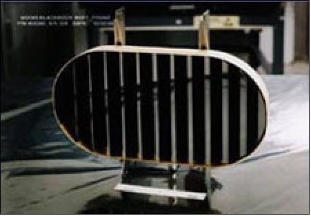
• Blackbody (BB) calibration of thermal bands on every scan (a v-groove blackbody)
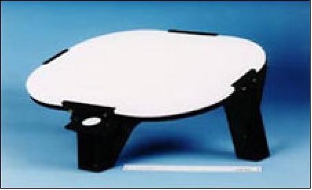
• Solar Diffuser (SD) reference
• Solar Diffuser Stability Monitor (SDSM)
The spectral mode of the SRCA device consists of a light source, a grating monochromator, and a beam collimator. The light source is a SIS (Spectral Integration Sphere) with lamps distributed inside. By combining the use of the spectral filters mounted on the filter wheel assembly and the grating monochromator, the SRCA is capable of performing spectral characterizations of the RSB (Reflective Solar Bands) ranging from 0.41 to 2.2 µm. Its spectral calibration is referenced to the ground equipment (SpMA) with high accuracy.
The SD/SDSM system is used for the RSB calibration and BB for the TEB (Thermal Emissive Bands) calibration. The SRCA is primarily used for the sensor's spectral (RSB only) and spatial (TEB and RSB) characterization. The RSB calibration is reflectance based using a sensor’s view of diffusely reflected sunlight from a solar diffuser (SD) plate with a known bi-directional reflectance and distribution function (BRDF). Because of the solar exposure onto the SD plate, its reflectance properties slowly degrade on-orbit.
The Blackbody is located in front of and slightly above the Scan Mirror, which views the BB with every revolution. The BB assembly provides a full-aperture radiometric calibration source of the MWIR and LWIR bands to within 1 percent absolute accuracy. It provides known radiance levels and is also used in the DC restore operation (a space-view signal level provides the second level for all bands in the two-point calibration). In normal operation the BB is kept at the instrument’s ambient temperature (nominally 273 K), though it is possible to heat and control the BB to 315K. Twelve sensors below the assembly's surface monitor its temperature. Each sensor is calibrated to National Institute of Standards & Technology (NIST) traceable standards, and can determine the temperature of the assembly to within ± 0.1 K.
To maintain the calibration and data quality, a solar diffuser stability monitor (SDSM) is used in tandem with the SD to track its degradation or BRDF changes. The SDSM system has a small integration sphere (SIS) with a single input aperture and nine filtered detectors. Each filter has a narrow spectral bandpass so that the change in reflectance is effectively monitored at nine discrete wavelengths between 0.4 µm and 1.0 µm. A three-position fold mirror enables the detectors to view sequentially a dark scene, direct sunlight, and illumination from the SD (Solar Diffuser). The direct sunlight is attenuated via a two-percent transmitting screen to keep the radiance within the dynamic range of the SDSM’s detector/amplifier combination.
MODIS product overview: MODIS provides global coverage every 1 to 2 days. It provides specific global survey data, which includes the following (some standard data products):
• Cloud mask: at 250 m and 1 km resolution by day and at night
• Aerosol concentration and optical properties: at 5 km resolution over oceans and 10 km over land during the day
• Cloud properties: characterized by optical thickness, effective particle radius, cloud droplet phase, cloud-top altitude, cloud-top temperature
• Vegetation and land-surface cover, conditions, and productivity, defined as:
- Vegetation indices corrected for atmospheric effects, soil, polarization, and directional effects
- Surface reflectance
- Land-cover type with identification and detection of change
- Net primary productivity, leaf-area index, and intercepted photosynthetically active radiation
• Snow and sea-ice cover and reflectance
• Surface temperature with 1 km resolution, day and night, with absolute accuracy goals of 0.3-0.5ºC for oceans and 1ºC for land surfaces.
• Ocean color: defined as ocean-leaving spectral radiance within 5% from 415-653 nm, based on adequate atmospheric correction from NIR sensor channels
• Concentration of chlorophyll-a within 35% from 0.05 to 50 mg/m3 for case 1 waters
• Chlorophyll fluorescence within 50% at surface water concentrations of 0.5 mg/m3 of chlorophyll-a.
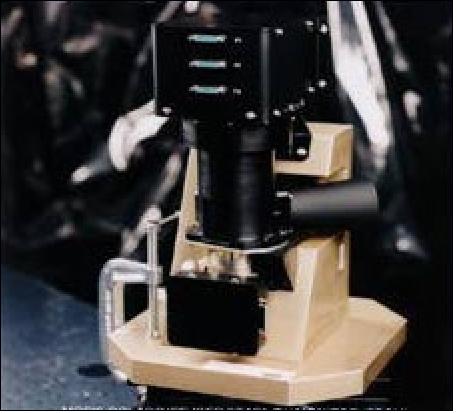
MOPITT (Measurement of Pollution in the Troposphere)
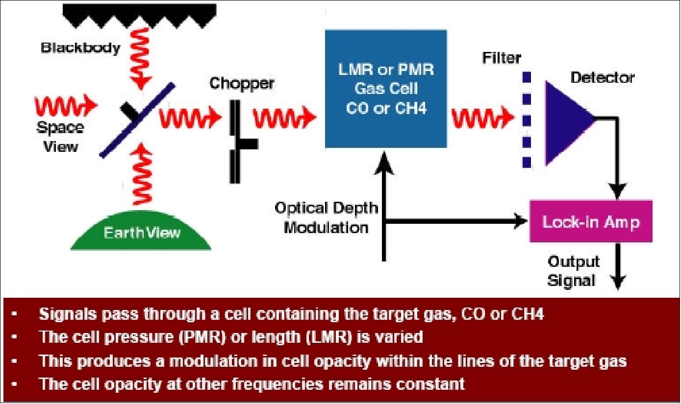
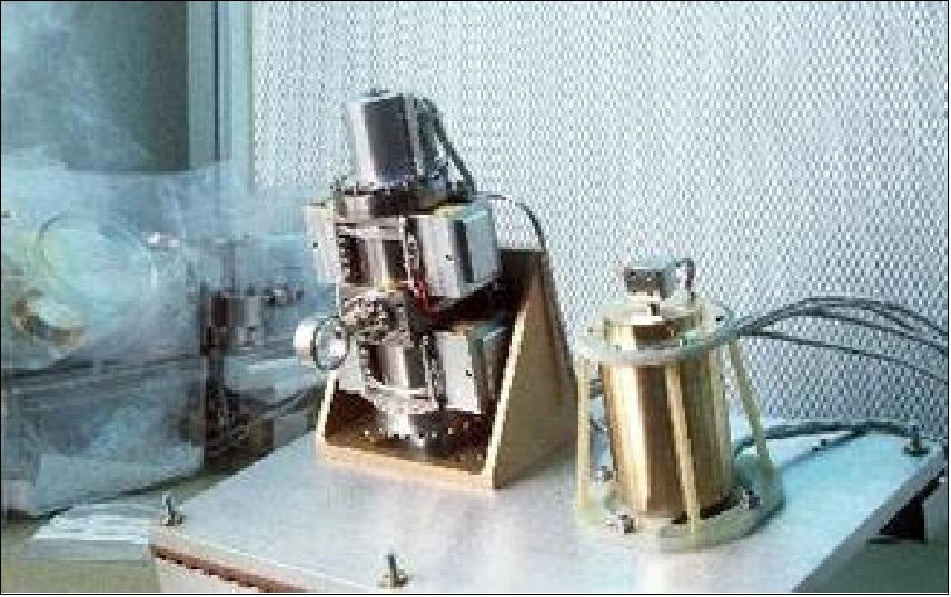
MOPITT is a Canadian sensor supported by CSA, built by COM DEV, Cambridge, Ontario (PI: J. R. Drummond, University of Toronto). The MOPITT instrument design is of MAPS (Measurements of Air Pollution from Space) heritage, flown on STS-2 (November 12.-14, 1981), then on STS-13 (October 5 -13, 1984), and then twice in 1994 (STS-59, STS-68). MOPITT is the first satellite sensor to use gas correlation spectroscopy (A technique to increase the sensitivity of the instrument to the gas of interest by separating out the regions of the spectrum where the gas has absorption lines and integrating the signal from just those regions. The specific wavelengths are located using a sample of the gas as a reference for the spectrum). By using correlation cells of differing pressures, some height resolution can be obtained. Thus MOPITT has multiple channels to provide height resolution, it also carries multiple channels to afford some redundancy. Definitions of acronyms in Table 10: LMC (Length Modulator Cell), PMC (Pressure Modulator Cell). 58) 59) 60) 61) 62) 63) 64) 65)
The CO profile measurements are made using upwelling thermal radiance in the 4.6 µm fundamental band. The troposphere is resolved into about four layers with approximately 3 km vertical resolution, 22 km horizontal resolution and 10% accuracy. Pressure Modulated Cells (PMCs) are used to view the upper layers whilst Length Modulated Cells (LMCs) are used for the lower troposphere measurements. By varying the cell pressures the modulators can be biased to view the different layers.
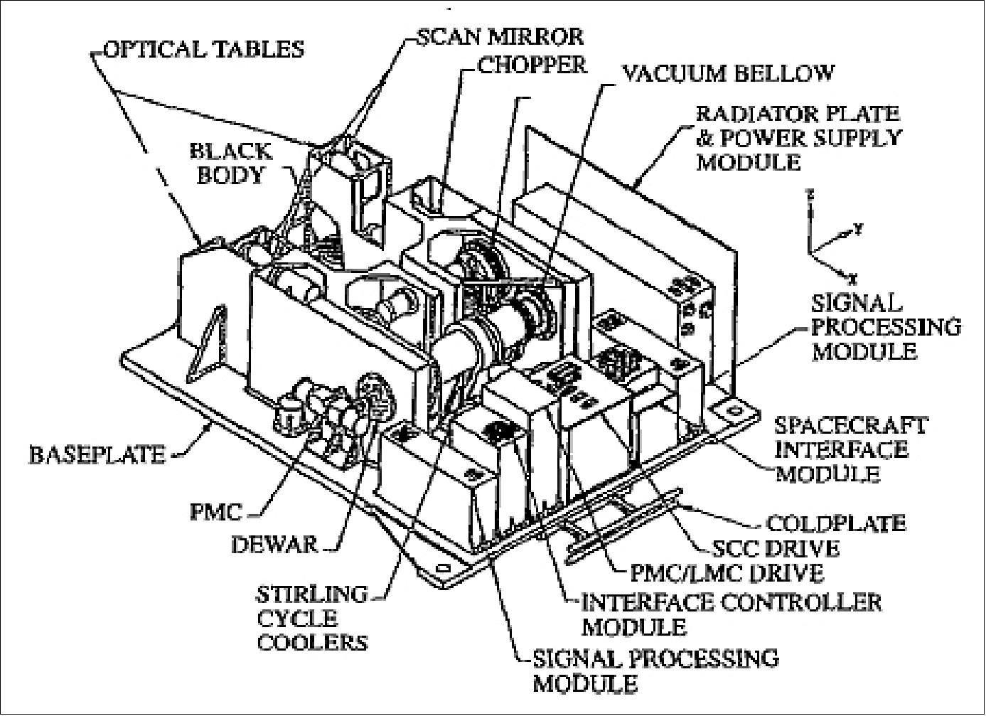
The MOPITT instrument contains four optical chains initiated by four scan mechanisms, which are split into eight independent channels. Each channel uses a technique known as correlation spectroscopy to perform the science measurements. This uses a sample of gas in the optical path. By performing synchronous demodulation of the detected infrared signal, the system functions as a complex filter, providing very good spectral resolution and good sensitivity by incorporating several molecular lines simultaneously.
Channel No | Cell type | Cell Pressure (kPa) | Center Wavelength (cm-1) | Spectral band constituent |
1 | LMC1 | 20 | 2166 (52) | CO thermal |
2 | LMC1 | 20 | 4285 (40) | CO solar |
3 | PMC1 | 7.5 | 2166 (52) | CO thermal |
4 | LMC2 | 80 | 4430 (140) | CH4 solar |
5 | LMC3 | 80 | 2166 (52) | CO thermal |
6 | LMC3 | 80 | 4285 (40) | CO solar |
7 | PMC2 | 3.75 | 2166 (52) | CO thermal |
8 | LMC4 | 80 | 4430 (140) | CH4 solar |
The instrument measures emitted and reflected infrared radiance in the atmospheric column. Analysis of these data permit retrieval of tropospheric CO profiles and total column CH4. Objective: study of how these gases interact with the surface, ocean, and biomass systems (distribution, transport, sources and sinks). Measurements are performed on the principle of correlation spectroscopy utilizing both pressure-modulated and length-modulated gas cells, with detectors at 2.3, 2.4, and 4.7 µm. Vertical profile of CO (carbon monoxide) and total column of CH4 (methane) are to be measured; CO concentration in 4 km layers with an accuracy of 10%; CH4 column abundance accuracy is 1%.
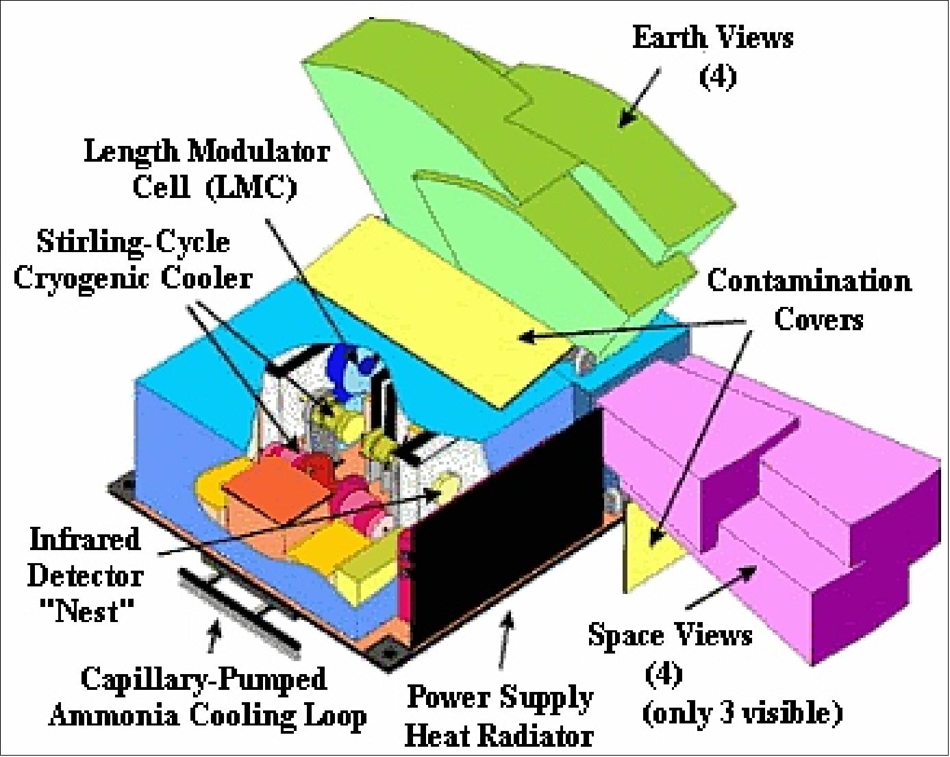
Swath width = 616 km, spatial resolution = 22 x 22 km; instrument mass = 182 kg; power = 243 W; duty cycle = 100%; data rate = 25 kbit/s; thermal control by an 80 K Stirling cycle cooler, capillary-pumped cold plate and passive radiation; thermal operating range = 25º C (instrument) and 100 K (detectors).
MOPITT is designed as a scanning instrument. IFOV = 1.8º x 1.8º (22 km x 22 km at nadir). The instrument scan line consists of 29 pixels, each at 1.8º increments. The maximum scan angle is 26.1º off-axis which is equivalent to a swath width of 640 km. - MOPITT data products include gridded retrievals of CH4 with a horizontal resolution of 22 km and a precision of 1%. Gridded CO soundings are retrieved with 10% accuracy in three vertical layers between 0 and 15 km. Three-dimensional maps to model global tropospheric chemistry.
The instrument is self-calibrating in orbit and performs a zero measurement every 120 seconds and a reference measurement every 660 seconds. The instrument operation is practically autonomous, requiring very little commanding to keep it within the mission profile at all times. 66)
MOPITT operations: MOPITT has suffered two anomalies since launch. On May 7, 2001 one of the two Stirling cycle coolers, which are used to keep the detectors at about 80 K, failed. The cooler fault compromised half of the instrument. After the fault, only channels 5, 6, 7, and 8 are delivering useful data. On Aug. 4, 2001 chopper 3 failed. Fortunately, it stopped in the completely open state, which permits to continue to use the data by adjusting the data processing algorithm accordingly.
EOS (Earth Observing System)
EOS is the centerpiece of NASA's Earth Science Enterprise (ESE). It consists of a science component and a data system supporting a coordinated series of polar-orbiting and low inclination satellites for long-term global observations of the land surface, biosphere, solid Earth, atmosphere, and oceans. 67) 68) 69) 70)
Background: The EOS program is a NASA initiative of the US Global Change Research Program (USGCRP). Planning for EOS began in the early 1980s, and an AO (Announcement of Opportunity) for the selection of instruments and science teams was issued in 1988. Early in 1990 NASA announced the selection of 30 instruments to be developed for EOS. Major budget constraints imposed by the US Congress forced the EOS program into a restructuring process in the time frame of 1991-92. In addition a rescoping of the EOS program occurred in 1992 leading to just half of the 1990 budget allocation (the HIRIS sensor was eliminated). The instruments adopted as part of the restructured/rescoped EOS program were chosen to address the key scientific issues associated with global climate change. This action reduced the required instruments to 17 that needed to fly by the year 2002 (six were deferred and seven instruments were deselected from the original 30). Furthermore, a shift occurred in the conceptual design of the EOS satellite platforms from “large observatories” to intermediate and smaller spacecraft that may be launched by smaller and existing launch vehicles. The EOS program experienced a further rebaselining process in 1994, due to a budget reduction of about 9%. This resulted in the cancellation of the combined EOS Radar and Laser Altimeter Mission (but rephasing the latter as two separate missions), deferring the development of some sensors and spreading the launch of missions by increasing the basic re-flight periods of missions from 5 to 6 years, and flying some EOS instruments on missions of partner space agencies (NASDA, RKA, CNES, ESA) in a framework of international cooperation. The EOS program includes instruments provided by international partners (ASTER, MOPITT, HSB, OMI) as well as an instrument developed by a joint US/UK partnership (HIRDLS).
The overall goal of the EOS program is to determine the extent, causes, and regional consequences of global climate change. The following science and policy priorities are defined for EOS observations (established by the EOS investigators working group and in coordination with the national and international Earth science community):
• Water and Energy Cycles: Cloud formation, dissipation, and radiative properties which influence the response of the atmosphere to greenhouse forcing, large-scale hydrology, evaporation
• Oceans: Exchange of energy, water, and chemicals between the ocean and atmosphere, and between the upper layers of the ocean and the deep ocean (including sea ice and formation of bottom water)
• Chemistry of the Troposphere and Lower Stratosphere: Links to the hydrologic cycle and ecosystems, transformations of greenhouse gases in the atmosphere, and interactions including climate change
• Land-Surface Hydrology and Ecosystem Processes: Improved estimates of runoff over the land surface and into the oceans. Sources and sinks of greenhouse gases. Exchange of moisture and energy between the land surface and the atmosphere. Changes in land cover
• Glaciers and Polar Ice Sheets: Predictions of sea level and global water balance
• Chemistry of the Middle and Upper Stratosphere: Chemical reactions, solar-atmosphere relations, and sources and sinks of radiatively important gases
• Solid Earth: Volcanoes and their role in climate change.
The original EOS mission elements (AM S/C series, PM S/C series, Chemistry S/C series) was redefined again in 1999. The EOS program space segment elements are now: Landsat-7, QuikSCAT, Terra, ACRIMSat, Aqua, Aura and ICESat.
Parameter | Terra (EOS/AM-1) S/C | Aqua (EOS/PM-1 S/C) |
Downlink center frequency | 8212.5 MHz | 8160 MHz |
EIRP | 14 W | 27.2 W |
Bandwidth | 26 MHz | 15 MHz |
Data modulation | OQPSK | SQPSK |
Data format | NRZ-L | NRZ-L |
I/Q power ratio (nominal) | 1:1 | 1:1 |
Operational duty cycle | 100% | 100% |
Antenna coverage from nadir | ±64º | ±64º |
Antenna polarization | RHCP | RHCP |
Data rate | 13 Mbit/s | 15 Mbit/s |
Data protocol standard | CCSDS | CCSDS |
Instrument data provided | MODIS | MODIS, AIRS, AMSU-A, CERES, HSB, AMSR-E |
EOS policy includes providing Direct Broadcast (DB) service to the user community; this applies to real-time MODIS data from the Terra spacecraft, as well as to the entire real-time data stream of the Aqua satellite. These data may be received by anyone with the appropriate receiving station, without charge. The broadcast data are transmitted in X-band. A 3 m antenna dish (minimum) should be sufficient for X-band data reception.
References
1) Special issue on EOS/AM-1 Platform, Instruments and Scientific Data, IEEE Transactions on Geoscience and Remote Sensing, Vol. 36, No 4, July 1998
3) http://library01.gsfc.nasa.gov/gdprojs/projinfo/terra.pdf
4) “Terra: Flagship of the Earth Observing System,” Press Kit, Nov. 1999, URL: http://www.nasa.gov/pdf/156293main_terra_press_kit.pdf
5) “TRW Completing Testing of EOS AM-1 Solar Array, First GaAs/Ge Flexible Blanket Solar Array,” May 13, 1997, URL: http://www.thefreelibrary.com/TRW+Completing+Testing+of+EOS+AM-1+Solar+Array,+First+GaAs%2FGe...-a019399069
6) M. J. Herriage, R. M. Kurland, C. D. Faust, E. M. Gaddy, D. J. Keys, “ EOS AM-1 GaAs/Ge flexible blanket solar array verification testprogram results,” Proceedings of the IECEC-97 (Energy Conversion Engineering Conference-1997), Vol. 1, pp.556-562, Honolulu, HI, USA, Sept. 27 to Aug. 1, 1997
7) D. J. Keys, “Earth Observing System (EOS) Terra spacecraft 120 volt power subsystem,” Proceedings of the IECEC-2000, Vol. 1, pp. 197-206, Las Vegas, NV, USA, July 24-28, 2000
8) J P. Chamoun, C. Connor, M. P. Hughes, R. P. Kozon, E. Moyer, R. E. Quinn, “Terra Spacecraft Deep Space Calibration Maneuver design and Execution,” Proceedings of the 27th annual AAS Guidance and Control Conference, Breckenridge, CO, Feb. 4-8, 2004, Guidance and Control 2004, Volume 118, ed. by J. D. Chapel and R. D. Culp, pp. 573-591, AAS 04-075
9) D. J. Keys, “Earth Observing System (EOS) TERRA spacecraft 120 volt power subsystem,” 35th Intersociety Energy Conversion Engineering Conference and Exhibit (IECEC), Las Vegas, NV, July 24-28, 2000, AIAA Collection of Technical Papers, Vol. 1 (A00-37701 10-44)
10) C. Filici, M. Suarez, “SAC-C Positioning in the Earth Morning Constellation,” Third International Workshop on Satellite Constellations and Formation Flying, Pisa, Italy, Feb. 24-26, 2003, pp. 57-62
11) ”Terra's Orbital Drift,” 19 November 2021, URL: https://www.youtube.com/watch?v=2OY3PHJ4bhc
12) ”Snow Blanket for the Andes,” NASA Earth Observatory, Image of the Day for 20 July 2022, URL: https://earthobservatory.nasa.gov/images/150100/snow-blanket-for-the-andes
13) ”Subpopulation of Greenland Polar Bears Found by NASA-Funded Study,” NASA Feature, 16 June 2022, URL: https://www.nasa.gov/feature/esnt/2022/subpopulation-of-greenland-polar-bears-found-by-nasa-funded-study
14) ”Peculiar Cloud Over the Caspian,” NASA Earth Observatory, Image of the Day for 16 June 2022, URL: https://earthobservatory.nasa.gov/images/149934/peculiar-cloud-over-the-caspian
15) ”How Aerosols Helped Untangle Carbon Monoxide Trends,” NASA Earth Observatory, Image of the Day for 27 May 2022, URL: https://earthobservatory.nasa.gov/images/149842/how-aerosols-helped-untangle-carbon-monoxide-trends
16) ”A Global Decline in Carbon Monoxide,” NASA Earth Observatory, Image of the Day for 26 May 2022, URL: https://earthobservatory.nasa.gov/images/149876/a-global-decline-in-carbon-monoxide
17) Rebecca R. Buchholz, Helen M. Worden, Mijeong Park, Gene Francis, Merritt N. Deeter, David P. Edwards, Louisa K. Emmons, Benjamin Gaubert, John Gille, Sara Martínez-Alonso, Wenfu Tang, Rajesh Kumar, James R. Drummond, Cathy Clerbaux, Maya George, Pierre-François Coheur, Daniel Hurtmans, Kevin W. Bowman, .. . Susan S. Kulawikl, ”Air pollution trends measured from Terra: CO and AOD over industrial, fire-prone, and background regions,” Remote Sensing of Environment, Volume 256, April 2021, 112275, https://doi.org/10.1016/j.rse.2020.112275
18) ”Red River Flooding is Worst in a Decade,” NASA Earth Observatory, Image of the Day for 12 May 2022, URL: https://earthobservatory.nasa.gov/images/149822/red-river-flooding-is-worst-in-a-decade
19) ”Assembling Australia,” NASA Earth Observatory, Image of the Day for 4 April 2022, URL: https://earthobservatory.nasa.gov/images/149654/assembling-australia
20) ”Breakup at Land Glacier,” NASA Earth Observatory, Image of the Day for 2 April 2022, URL: https://earthobservatory.nasa.gov/images/149650/breakup-at-land-glacier
21) ”Dusty Storm Clouds Over Europe,” NASA Earth Observatory, Image of the Day for 31 March 2022, URL: https://earthobservatory.nasa.gov/images/149645/dusty-storm-clouds-over-europe
22) Yvette Smith, ”3.6 Billion Years in Pastel Colors,” NASA Feature, 9 March 2022, URL: https://www.nasa.gov/image-feature/36-billion-years-in-pastel-colors
23) ”Antarctic Berg Grounded for Decades,” NASA Earth Observatory, Image of the Day for 1 March 2022, URL: https://earthobservatory.nasa.gov/images/149522/antarctic-berg-grounded-for-decades?src=eoa-iotd
24) ”Bracing for Batsirai,” NASA Earth Observatory, Image of the Day for 5 February 2022, URL: https://earthobservatory.nasa.gov/images/149420/bracing-for-batsirai
25) ”A Modern Lake in an Ancient Crater,” NASA Earth Observatory, Image of the Day for 4 February 2022, URL: https://earthobservatory.nasa.gov/images/149414/a-modern-lake-in-an-ancient-crater
26) ”Coloring the South Atlantic,” NASA Earth Observatory, Image of the Day for 28 January 2022, URL: https://earthobservatory.nasa.gov/images/149384/coloring-the-south-atlantic
27) ”Great Lakes Cloud Streets,” NASA Earth Observatory, Image of the Day for 17 January 2022, URL:https://earthobservatory.nasa.gov/images/149339/great-lakes-cloud-streets
28) ”Failed Rainy Seasons Bring Famine Concerns to Eastern Africa,” NASA Earth Observatory, Image of the Day for 7 January 2022, URL: https://earthobservatory.nasa.gov/images/149294/failed-rainy-seasons-bring-famine-concerns-to-eastern-africa
29) ”A Winter Haze Over China,” NASA Earth Observatory, Image of the Day for 6 January 2022, URL: https://earthobservatory.nasa.gov/images/149291/a-winter-haze-over-china
30) ”Mid-Atlantic Snow Band,” NASA Earth Observatory, 4 January 2022, URL: https://earthobservatory.nasa.gov/images/149288/mid-atlantic-snow-band
31) ”Cornwall Clay Mines,” NASA Earth Observatory, Image of the Day for 03 January 2022, URL: https://earthobservatory.nasa.gov/images/149263/cornwall-clay-mines
32) Y. Yamaguchi, A. B. Kahle, H. Tsu, T. Kawakami, M. Pniel, “Overview of Advanced Spaceborne Thermal Emission and Reflection Radiometer (ASTER),” IEEE Transactions on Geoscience and Remote Sensing, Vol. 36,, pp. 1062-1071, 1998.
33) http://asterweb.jpl.nasa.gov/
34) ASTER, EOS Reference Handbook, 1999, pp. 102-105
35) Y. Yamaguchi, H. Tsu, H. Fujisada, “Scientific basis of ASTER instrument design,” Proceedings of SPIE (The International Society for Optical Engineering), Vol. 1939, 1993, pp. 150-160
36) M. Abrams, S. Hook, “ASTER User Handbook,” Version 1
37) Y. Yamaguchi, H. Fujisada, A. B. Kahle, H. Tsu, M. Kato, H. Watanabe, I. Sato, M. Kudoh, “ASTER Instrument Performance, Operation Status, and Application to Earth Sciences,” Proceedings of IGARSS 2001, Vol. 3, pp.:1215 - 1216, Sydney, Australia, July 9-13, 2001
38) M. Kawada, H. Akao, M. Kobayashi, et al., “Performance evaluation of ASTER cryocooler in orbit,” Proceedings of SPIE, Vol. 4881, 9th International Symposium on Remote Sensing, Aghia Pelagia, Crete, Greece, Sept. 23-27, 2002
39) http://asterweb.jpl.nasa.gov/instrument.asp
40) H. Fujisada, M. Ono, “Overview of ASTER design concept,” in. Future European and Japanese Remote Sensing Sensors and Programs,” SPIE Vol 1490, Bellingham, WA, April 1-2, 1991, pp. 244-254
41) NASA/LaRC CERES brochure, URL: http://ceres.larc.nasa.gov/press_releases/images/brochure.pdf
42) “CERES on Terra,” NASA, URL: http://asd-www.larc.nasa.gov/ceres/terra/
43) B. R. Barkstrom, B. A. Wielicki, “Bruce R. Barkstrom and Bruce A. Wielicki,” Proceedings of IGARSS 2000, Honolulu, Hawaii, USA, July 24-28, 2000
44) http://science.larc.nasa.gov/ceres/index.html
45) R. S. Wilson, R. B. Lee, et al., “On-orbit solar calibrations using the Aqua Clouds and Earth's Radiant Energy System (CERES) in-flight calibration system,” Proceedings of SPIE, Vol. 5151, 2003, pp. 288-299
46) D. J. Diner, J. C. Beckert, G. W. Bothwell, J. I. Rodriguez, (2002). “Performance of the MISR Instrument During Its First 20 Months in Earth Orbit.,” IEEE Transactions on. Geoscience and Remote Sensing. Vol. 40, No 7, July 2002, pp. 1449-1466
47) C. J. Bruegge, D. J. Diner, “Instrument verification tests on the Multi-angle Imaging SpectroRadiometer (MISR),”. In Earth Observing System II, Proceedings of SPIE, Vol. 3117, San Diego, CA, July. 1997
48) D. J. Diner, C.J. Bruegge, J. V., G. W. Bothwell, E. D. Danielson, V. G. Ford, L. E. Hovland, K. L. Jones, M. L. White, “A Multi-angle Imaging SpectroRadiometer for terrestrial remote sensing from the Earth Observing System,” International. Journal of Imaging Systems and Technology, Vol. 3, 1991, pp. 92-107
49) http://misr.jpl.nasa.gov/Mission/
50) Rebecca Lindsey, David Herring, “MODIS brochure,” NASA/GSFC, URL: http://modis.gsfc.nasa.gov/about/media/modis_brochure.pdf
51) http://modis.gsfc.nasa.gov/
52) C. Schueler, W. L. Barnes, “Next-Generation MODIS for Polar Operational Environmental Satellites,” Journal of Atmospheric and Oceanic Technology, Vol. 15, Issue 2, April 1998, pp.430-439, URL: http://journals.ametsoc.org/doi/pdf/10.1175/1520-0426%281998%29015%3C0430%3ANGMFPO%3E2.0.CO%3B2
53) R. Wolfe, “MODIS Calibration, Geolocation and Production,” EOS Snow and Ice Workshop, November 15, 2004, URL: http://nsidc.org/news/events/eos_workshop04/presentations/wolfe.ppt
54) Information provided by C. Schueler and J. Thunen of Hughes SBRC (now Raytheon SBRS)
55) X. Xiong, N. Che, B. Guenther, W. L. Barnes, V. V. Salomonson, “Five Years of Terra MODIS On-Orbit Spectral Characterization,” Proceedings of SPIE Conference Optics and Photonics 2005, San Diego, CA, USA, July 31-Aug. 4, 2005, Vol. 5882
56) W. Barnes, X. Xiong, T. Salerno, B. Breen, C. Salo, “Operational activities and on-orbit performance of Terra MODIS on-board calibrators,” Proceedings of SPIE Conference Optics and Photonics 2005, San Diego, CA, USA, July 31-Aug. 4, 2005, Vol. 5882
57) http://modis.gsfc.nasa.gov/about/components.php
58) http://www.atmosp.physics.utoronto.ca/MOPITT/home.html
59) J. R. Drummond, “MOPITT: 12 Years of Planning and 2.5 Years of Operations,” Proceedings of IGARSS 2002, Toronto, Canada, June 24-28, 2002
60) R. Deschambault, J. Hackett, D. Henry, T. Girard, F. Nichitiu, J. Zou, R. Irvine, J. R. Drummond, “MOPITT Flight Operations,” Proceedings of IGARSS 2002, Toronto, Canada, June 24-28, 2002
61) L. Emmons, D. Edwards, J. Gille, J.-L. Attié, M. Deeter, J. Warner, D. Ziskin, J. Drummond, E. McKernan, L. Yurganov, L. Jounot, B. Tolton, “MOPITT Validation Summary,” July 2001
62) J. R. Drummond, P. L. Bailey, G. Brasseur, G. R. Davis, J. C. Gille, G. D. Peskett, H. K. Reichle, N. Roulet, G. S. Mand, J. C. McConnell, “Early Mission Planning for the MOPITT Instrument,” URL: http://www.atmosp.physics.utoronto.ca/MOPITT/mission.pdf
63) J. R. Drummond, G. S. Mand, “The Measurement of Pollution in the Troposphere (MOPITT) Instrument: Overall Performance and Calibration Requirements,” Journal of Atmospheric and Oceanic Technology, Vol. 13, 1996, pp. 314-320,
64) D. Caldwell, J. Hackett, A. S. Gibson, J. R. Drummond, F. Nichitiu, “The Design and Flight Performance of the MOPITT Instrument Mechanisms,” Proceedings of the 11th European Space Mechanisms and Tribology Symposium, ESMATS 2005, 21-23 September 2005, Lucerne, Switzerland. Edited by B. Warmbein. ESA SP-591, Noordwijk, Netherlands: ESA Publications Division, ISBN 92-9092-902-2, 2005, pp. 99 - 106, URL: http://articles.adsabs.harvard.edu/full/seri/ESASP/0591//0000099.000.html
65) http://eospso.gsfc.nasa.gov/ftp_docs/MOPITT%20broch.pdf
66) J. Zou, F. Nichitiu, J. R. Drummond, “The Calibration of the MOPITT instrument,” Proceedings of IGARSS 2002, Toronto, Canada, June 24-28, 2002
67) G. Asrar, R. Greenstone (editors), “MTPE/EOS Reference Handbook 1995,” NASA/GSFC
68) “Earth Observing System,” Reference Handbook 1990, and 1991, NASA/GSFC
69) “Optical Remote Sensing of the Atmosphere,” 1990 Technical Digest Series of the Optical Society of America, Volume 4, pp. 23-58
70) G. Asrar, D. J. Dokken, “EOS Reference Handbook,” March 1993, NASA
Spacecraft Launch Mission Status Sensor Complement EOS References Back to top