Landsat-8/LDCM
EO
Atmosphere
Ocean
Cloud type, amount and cloud top temperature
Landsat-8, launched in February 2013, is the eighth satellite in NASA’s Landsat spacecraft series, and the first of the Landsat Data Continuity Mission (LDCM). Operated by the United States Geological Survey (USGS), this collaborative mission aims to collect and archive thermal and multispectral image data whilst ensuring consistency with previous Landsat mission data.
Quick facts
Overview
| Mission type | EO |
| Agency | NASA, USGS |
| Mission status | Operational (extended) |
| Launch date | 11 Feb 2013 |
| Measurement domain | Atmosphere, Ocean, Land, Snow & Ice |
| Measurement category | Cloud type, amount and cloud top temperature, Ocean colour/biology, Multi-purpose imagery (ocean), Radiation budget, Multi-purpose imagery (land), Surface temperature (land), Vegetation, Albedo and reflectance, Ocean topography/currents, Sea ice cover, edge and thickness, Snow cover, edge and depth, Inland Waters |
| Measurement detailed | Ocean imagery and water leaving spectral radiance, Ocean chlorophyll concentration, Cloud cover, Cloud imagery, Land surface imagery, Fire temperature, Vegetation type, Fire fractional cover, Earth surface albedo, Short-wave Earth surface bi-directional reflectance, Leaf Area Index (LAI), Land cover, Land surface temperature, Sea-ice cover, Snow cover, Normalized Differential Vegetation Index (NDVI), Iceberg fractional cover, Bathymetry, Fraction of Absorbed PAR (FAPAR), Glacier motion, Glacier cover, Sea-ice surface temperature, Above Ground Biomass (AGB), Active Fire Detection, Long-wave Earth surface emissivity, Permafrost, Evapotranspiration, Cloud mask, Surface Water Extent, Mineral Type |
| Instruments | TIRS, OLI |
| Instrument type | Imaging multi-spectral radiometers (vis/IR) |
| CEOS EO Handbook | See Landsat-8/LDCM summary |
Related Resources
Summary
Mission Capabilities
Landsat-8 features an Operational Land Imager (OLI) and a Thermal Infrared Sensor instrument (TIRS), which together replace the Enhanced Thematic Mapper Plus (ETM+) instrument on the preceding satellite (Landsat-7). Developed by Ball Aerospace Technology Corporation (BATC), the OLI instrument is a multispectral and moderate resolution imager. OLI has nine spectral bands covering a spectral range from 433 - 2300 nm, including five in the visible and near infrared spectrum (NVIR), three in the short-wave infrared spectrum (SWIR), and one panchromatic image (PAN) band for image sharpening. The thermal imaging band (TIR) was removed due to the extra cost of active cooling. The NVIR bands are primarily used for aerosol, pigments and coastal zone monitoring, whilst the SWIR bands are used for foliage, mineral and litter observation. The SWIR band (1360 - 1390 nm) is used for detecting cirrus clouds.
TIRS is a Quantum Well Infrared Photodetector (QWIP) based instrument that provides continuity for two infrared bands not imaged by OLI. These thermal imaging bands provide data used to measure evapotranspiration, map urban heat fluxes, monitor lake thermal plumes, identify mosquito breeding areas and provide cloud measurements.
Performance Specifications
The sensors onboard feature pushbroom architecture, making it more geometrically stable but requiring terrain selection to ensure accurate band registration. The spacecraft is able to achieve a 185 km swath width with a 15 degree field of view functioning in the pushbroom sample collection method. Moderate spatial, spectral and thermal resolutions are sufficient to characterise and understand the causes and consequences of land cover/land use change. A spatial resolution of 15m PAN, 30m for VNIR/SWIR and a thermal resolution of 100m coincides with the scale of human activities, thus allowing for clearer observation of human impact on the planet’s various systems.
The satellite undergoes a sun-synchronous orbit at an altitude of 705 km with a period of 99 minutes and repeat coverage of 16 days.
Space and Hardware Components
The Landsat-8 spacecraft uses a nadir-pointing, three-axis stabilised bus built by GDAIS (General Dynamics Advanced Information Systems) referred to as SA-200HP. It features an Electric Power Subsystem using triple junction solar panels, an Altitude Determination & Control Subsystem, Command & Data Handling system and propulsion system.
The spacecraft has a mass of 2780 kg and a design life of 5 years, although it contains onboard consumables to support 10 years of operation.
Landsat-8 / LDCM (Landsat Data Continuity Mission)
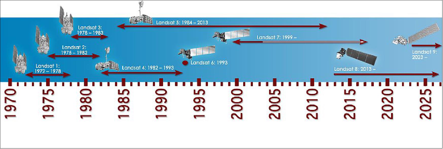
The Landsat spacecraft series of NASA represents the longest continuous Earth imaging program in history, starting with the launch of Landsat-1 in 1972 through Landsat-7 with the ETM+ imager (launch April 15, 19la99). With the evolution of the program has come an increased emphasis on the scientific utility of the data accompanied by more stringent requirements for instrument and data characterisation, calibration and validation. This trend continues with LDCM, the next mission in the Landsat sequence. The enhancements of the Landsat-7 system, e.g., more on-board calibration hardware and an image assessment system and personnel, have been retained and improved, where required, for LDCM. Aspects of the calibration requirements are spread throughout the mission, including the instrument and its characterisation, the spacecraft, operations and the ground system. 1) 2)
The following are the major mission objectives: 3)
• Collect and archive moderate-resolution, reflective multispectral image data affording seasonal coverage of the global land mass for a period of no less than five years.
• Collect and archive moderate-resolution, thermal multispectral image data affording seasonal coverage of the global land mass for a period of no less than three years.
• Ensure that LDCM data are sufficiently consistent with data from the earlier Landsat missions, in terms of acquisition geometry, calibration, coverage characteristics, spectral and spatial characteristics, output product quality, and data availability to permit studies of land cover and land use change over multi-decadal periods.
• Distribute standard LDCM data products to users on a nondiscriminatory basis and at no cost to the users.
Background: In 2002, the Landsat program had its 30th anniversary of providing satellite remote sensing information to the world; indeed a record history of service with the longest continuous spaceborne optical medium-resolution imaging dataset available anywhere. The imagery has been and is being used for a multitude of land surface monitoring tasks covering a broad spectrum of resource management and global change issues and applications.
In 1992 the US Congress noted that Landsat commercialisation had not worked and brought Landsat back into the government resulting in the launches of Landsat 6 (which failed on launch) and Landsat 7. However there was still much conflict within the government over how to continue the program.
In view of the outstanding value of the data to the user community as a whole, NASA and USGS (United States Geological Survey) were working together (planning, rule definition, forum of ideas and discussion among all parties involved, coordination) on the next generation of the Landsat series satellites, referred to as LDCM (Landsat Data Continuity Mission). The overall timeline foresaw a formulation phase until early 2003, followed by an implementation phase until 2006. The goal was to acquire the first LDCM imagery in 2007 - to ensure the continuity of the Landsat dataset [185 km swath width, 15 m resolution (Pan) and a new set of spectral bands]. 4) 5) 6) 7) 8) 9) 10) 11)
The LDCM project suffered some setbacks on its way to realisation resulting in considerable delays:
• An initial major programmatic objective of LDCM was to explore the use of imagery purchases from a commercial satellite system in the next phase of the Landsat program. In March 2002, NASA awarded two study contracts to: a) Resource21 LLC. of Englewood, CO, and b) DigitalGlobe Inc. of Longmont, CO. The aim was to formulate a proper requirements set and an implementation scenario (options) for LDCM. NASA envisioned a PPP (Public Private Partnership) program in which the satellite system was going to be owned and operated commercially. A contract was to be awarded in the spring of 2003. - However, it turned out that DigitalGlobe lost interest and dropped out of the race. And the bid of Resource21 turned out to be too high for NASA to be considered.
• In 2004, NASA was directed by the OSTP (Office of Science and Technology Policy) to fly a Landsat instrument on the new NPOESS satellite series of NOAA.
• In Dec. 2005, a memorandum with the tittle “Landsat Data Continuity Strategy Adjustment” was released by the OSTP which directed NASA to acquire a free-flyer spacecraft for LDCM - thus, superseding the previous direction to fly a Landsat sensor on NPOESS. 12)
However, the matter was not resolved until 2007 when it was determined that NASA would procure the next mission, the LDCM, and that the USGS would operate it as well as determine all future Earth observation missions. This decision means that Earth observation has found a home in an operating agency whose mission is directly concerned with the mapping and analysis of the Earth’s surface allowing NASA to focus on advancing space technologies and the future of man in space.
Overall science objectives of the LDCM imager observations are:
• To permit change detection analysis and to ensure consistency of the LDCM data with the Landsat series data
• To provide global coverage of the Earth's land surfaces on a seasonal basis
• To acquire imagery at spatial, spectral and temporal resolutions sufficient to characterise and understand the causes and consequences of change
• To make the data available to the user community.
The procurement approach for the LDCM project represents a departure from a conventional NASA mission. NASA traditionally specifies the design of the spacecraft, instruments, and ground systems acquiring data for its Earth science missions. For LDCM, NASA and USGS (the science and technology agency of the Department of the Interior, DOI) have instead specified the content, quantity, and characteristics of data to be delivered.
“The Landsat series of satellites is a cornerstone of our Earth observing capability. The world relies on Landsat data to detect and measure land cover/land use change, the health of ecosystems, and water availability,” NASA Administrator Charles Bolden told the Subcommittee on Space Committee on Science, Space and Technology U.S House of Representatives in April 2015.
“With a launch in 2023, Landsat-9 would propel the program past 50 years of collecting global land cover data,” said Jeffrey Masek, Landsat-9 Project Scientist at Goddard. “That’s the hallmark of Landsat: the longer the satellites view the Earth, the more phenomena you can observe and understand. We see changing areas of irrigated agriculture worldwide, systemic conversion of forest to pasture – activities where either human pressures or natural environmental pressures are causing the shifts in land use over decades.”
Landsat-8 successfully launched on Feb. 11, 2013 and the Landsat data archive continues to expand. — Landsat-9 was announced on April 16, 2015. The launch is planned for 2023. 14)
Dec. 31, 2015: NASA has awarded a sole source letter contract to BACT (Ball Aerospace & Technologies Corporation), Boulder, Colo., to build the OLI-2 (Operational Land Imager-2) instrument for the Landsat-9 project. 15)
Spacecraft
In April 2008, NASA selected GDAIS (General Dynamics Advanced Information Systems), Inc., Gilbert, AZ, to build the LDCM spacecraft on a fixed price contract. An option provides for the inclusion of a second payload instrument. LDCM is a NASA/USGS partnership mission with the following responsibilities: 16) 17) 18) 19)
• NASA is providing the LDCM spacecraft, the instruments, the launch vehicle, and the mission operations element of the ground system. NASA will also manage the space segment early on-orbit evaluation phase -from launch to acceptance.
• USGS is providing the mission operations center and ground processing systems (including archive and data networks), as well as the flight operations team. USGS will also co-chair and fund the Landsat science team.
In April 2010, OSC (Orbital Sciences Corporation) of Dulles VA acquired GDAIS. Hence, OSC will continue to manufacture and integrate the LDCM program as outlined by GDAIS. Already in Dec. 2009, GDAIS successfully completed the CDR (Critical Design Review) of LDCM for NASA/GSFC. 20) 21)

The spacecraft is 3-axis stabilised (zero momentum biased). The ADCS (Attitude Determination and Control Subsystem) employs six reaction wheels, three torque rods and thrusters as actuators. Attitude is sensed with three precision star trackers (2 of 3 star trackers are active), a redundant SIRU (Scalable Inertial Reference Unit), twelve coarse sun sensors, redundant GPS receivers (Viceroy), and two TAMs (Three Axis Magnetometers).
- Attitude control error (3σ): ≤ 30 µrad
- Attitude knowledge error (3σ): ≤ 46 µrad
- Attitude knowledge stability (3σ): ≤ 0.12 µrad in 2.5 seconds; ≤ 1.45 µrad in 30 seconds
- Slew time: 180º any axis: ≤ 14 minutes, including settling; 15º roll: ≤ 4.5 minutes, including settling.
Key aspects of the satellite performance related to imager calibration and validation are pointing, stability and maneuverability. Pointing and stability affect geometric performance; maneuverability allows data acquisitions for calibration using the sun, moon and stars. For LDCM, an off nadir acquisition capability is included (up to 1 path off nadir) for imaging high priority targets (event monitoring capability).
Also, the spacecraft pointing capability will allow the calibration of the OLI using the sun (roughly weekly), the moon (monthly), stars (during commissioning) and the Earth (at 90° from normal orientation, a.k.a., side slither) quarterly. The solar calibration will be used for OLI absolute and relative calibration, the moon for trending the stability of the OLI response, the stars will be used for Line of Sight determination and the side slither will be an alternate OLI and relative gain determination methodology. 22) 23)
C&DH (Command & Data Handling) subsystem: The C&DH subsystem uses a standard cPCI backplane RAD750 CPU. The MIL-STD-1553B data bus is used for onboard ADCS, C&DH functions and instrument communications. The SSR (Solid State Recorder) provides a storage capacity of 4 Tbit @ BOL and 3.1 Tbit @ EOL.
The C&DH subsystem provides the mission data interfaces between instruments, the SSR, and the X-band transmitter. The C&DH subsystem consists of an IEM (Integrated Electronics Module), a PIE (Payload Interface Electronics), the SSR, and two OCXO (Oven Controlled Crystal Oscillators).
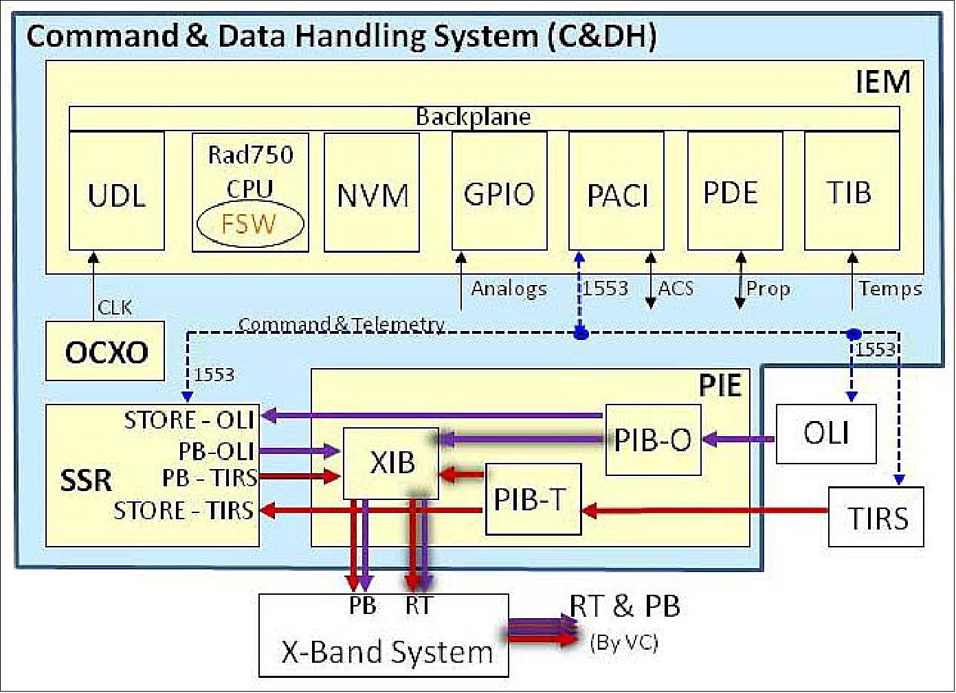
- The IEM subsystem provides the command and data handling function for the observatory, including mission data management between the PIE and SSR using FSW on the Rad750 processor. The IEM is block redundant with cross strapped interfaces for command and telemetry management, attitude control, SOH (State of Health) data and ancillary data processing, and for controlling image collection and file downlinks to the ground.
- The SSR subsystem provides for mission data and spacecraft SOH storage during all mission operations. The OCXO provides a stable, accurate time base for ADCS fine pointing.
- The C&DH accepts encrypted ground commands for immediate execution or for storage in the FSW file system using the relative time and absolute time command sequences (RTS, ATS respectfully). The commanding interface is connected to the uplink of each S-band transceiver, providing for cross-strapped redundancy to the C&DH. All commands are verified onboard prior to execution. Real-time commands are executed upon reception, while stored commands are placed in the FSW file system and executed under control of the FSW. Command counters and execution history are maintained by the C&DH FSW and reported in SOH telemetry.
- The IEM provides the command and housekeeping telemetry interfaces between the payload instruments and the ADCS components using a MIL-STD-1553B serial data bus and discrete control and monitoring interfaces. The C&DH provides the command and housekeeping interfaces between the CCU (Charge Control Unit), LCU (Load Control Unit) , and the PIE boxes.
- The PIE is the one of the key electrical system interfaces and mission data processing systems between the instruments, the spacecraft C&DH, SSR, and RF communications to the ground. The PIE contains the PIB (Payload Interface Boards ) for OLI (PIB-O) and TIRS (PIB-T).
Each PIB contains an assortment of specialised FPGAs (Field Programmable Gate Arrays) and ASICs, and each accepts instrument image data across the HSSDB for C&DH processing. A RS-485 communication bus collects SOH and ACS ancillary data for interleaving with the image data.
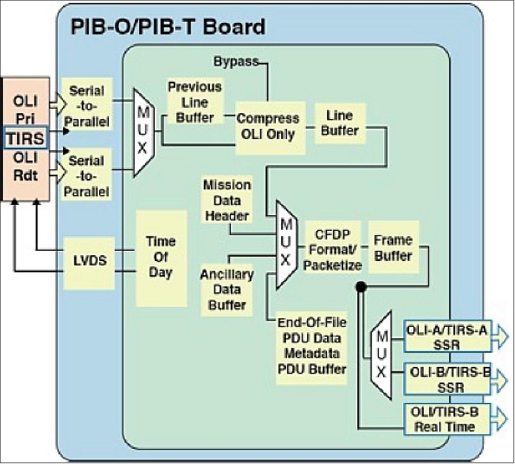
- Data compression: Only the OLI data, sent through the PIB-O interface, implements lossless compression, by utilising a pre-processor and entropy encoder in the USES ASIC. The compression can be enabled or bypassed on an image-by-image basis. When compression is enabled the first image line of each 1 GB file is uncompressed to provide a reference line to start that file. A reference line is generated every 1,024 lines (about every 4 seconds) to support real-time ground contacts to begin receiving data in the middle of a file and decompressing the image with the reception of a reference line.
- XIB (X-band Interface Board): The XIB is the C&DH interface between the PIE, SSR, and X-band transmitter, with the functional data path shown in Figure 6.
The XIB receives real-time data from the PIE PIB-O and PIB-T and receives stored data from the SSR via the 2 playback ports. The XIB sends mission data to the X-band transmitter via a parallel LVDS interface. The XIB receives a clock from the X-band transmitter to determine the data transfer rates between the XIB and the transmitter to maintain a 384 Mbit/s downlink. The XIB receives OLI realtime data from the PIB-O board, and TIRS real-time data from the PIB-T board across the backplane. The SSR data from the PIB-O and PIB-T interfaces are multiplexed and sent to the X-Band transmitter through parallel LVDS byte-wide interfaces.

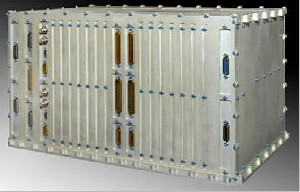
- SSR (Solid Ste Recorder): The SSR is designed with radiation hard ASIC controllers, and up-screened commercial grade 4GB SDRAM (Synchronous Dynamic Random Access Memory) memory devices. Protection against on-orbit radiation induced errors is provided by a Reed-Solomon EDAC (Error Detection and Correction) algorithm. The SSR provides the primary means for storing all image, ancillary, and state of health data using a file management architecture. Manufactured in a single mechanical chassis, containing a total of 14 memory boards, the system provides fully redundant sides and interfaces to the spacecraft C&DH.
The spacecraft FSW (Flight Software) plays an integral role in the management of the file directory system for recording and file playback. FSW creates file attributes for identifier, size, priority, protection based upon instructions from the ground defining the length of imaging in the interval request, and its associated priority. FSW also maintains the file directory, and creates the ordered lists for autonomous playback based upon image priority. FSW automatically updates and maintains the spacecraft directory while recording or performing playback, and it periodically updates the SSR FSW directory when no recording is occurring to synchronise the two directories (Ref. 107).
TCS (Thermal Control Subsystem): The TCS uses standard Kapton etched-foil strip heaters. In general, a passive, cold-biased system is used for the spacecraft. Multi-layer insulation on spacecraft and payload as required. A deep space view is provided for the instrument radiators.
EPS (Electric Power Subsystem): The EPS consists of a single deployable solar array with single-axis articulation capability and with a stepping gimbal. Triple-junction solar cells are being used providing a power of 4300 W @ EOL. The NiH2 battery has a capacity of 125 Ah. Use of unregulated 22-36 V power bus.
The onboard propulsion subsystem provides a total velocity change of ΔV = 334 m/s using eight 22 N thrusters for insertion error correction, altitude adjustments, attitude recovery, EOL disposal, and other operational maintenance as necessary.
The spacecraft has a launch mass of 2780 kg (1512 kg dry mass). The mission design life is 5 years; the onboard consumable supply (386 kg of hydrazine) will last for 10 years of operations.
Spacecraft platform | SA-200HP (High Performance) bus |
Spacecraft mass | Launch mass of 2780 kg; dry mass of 1512 kg |
Spacecraft design life | 5 years; the onboard consumable supply (386 kg of hydrazine) will last for 10 years of operations |
EPS (Electric Power Subsystem) | - Power: 4.3 kW @ EOL (End of Life) |
ADCS (Attitude Determination & | - Actuation: 6 reaction wheels and 3 torque rods |
C&DH (Command & Data Handling) | - Standard cPCI backplane RAD750 CPU |
Propulsion subsystem | - Total velocity change of ΔV = 334 m/s using eight 22 N thrusters |
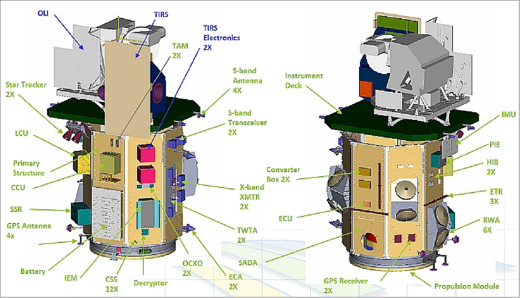
RF communications: Earth coverage antennas are being used for all data links. The X-band downlink uses lossless compression and spectral filtering. The payload data rate is 440 Mbit/s. The X-band RF system consists of the X-band transmitter, TWTA (Travelling Wave Tube Amplifier), DSN (Deep Space Network) filter, and an ECA (Earth Coverage Antenna). The serial data output is set at 440.825 Mbit/s and is up-converted to 8200.5 MHz. The TWTA amplifies the signal such that the output of the DSN filter is 62 W. The DSN filter maintains the signal’s spectral compliance. An ECA provides nadir full simultaneous coverage, utilising 120º half-power beamwidth, for all in view ground sites below the spacecraft's current position with no gimbal or actuation system. The system is designed to handle up to 35 separate ground contacts per day as forecasted by the DRC-16 (Design Reference Case-16).
The X-band transmitter is a single customised unit, including the LDPC FEC algorithms, the modulator, and up converter circuits. The transmitter uses a local TXCO (Thermally Controlled Crystal Oscillator) as a clock source for tight spectral quality and minimum data jitter. This clock is provided to the PIE XIB to clock mission data up to a 384Mbit/s data rate to the transmitter. The X-band transmitter includes an on-board synthesised clock operating at 441.625 Mbit/s coded data rate using the local 48 MHz clock as a reference. Using the on-board FIFO buffer, this architecture provides a continuous data flow through the transmitter (Ref. 107).
The S-band is used for all TT&C functions. The S-band uplink is encrypted providing data rates of 1, 32, and 64 kbit/s. The S-band downlink offers data rates of 2, 16, 32, RTSOH; 1 Mbit/s SSOH/RTSOH GN; 1 kbit/s RTSOH SN. Redundant pairs of S-band omni’s provide transmit/receive coverage in any orientation. The S-band is provided through a typical S-band transceiver, with TDRSS (Tracking and Data Relay Satellite System) capability for use during launch and early orbit and in case of spacecraft emergencies.
Onboard data transmission from an earth-coverage antenna:
• Real-time data received from PIE (Payload Interface Electronics) equipment
• Play-back data from SSR (Solid State Recorder)
• To three LGN (LDCM Ground Network) stations
- NOAA Interagency Agreement (IA) to use Gilmore Creek Station (GLC) near Fairbanks, AK
- Landsat Ground Station (LGS) at USGS/EROS near Sioux Falls, SD
- NASA contract with KSAT for Svalbard; options for operational use by USGS (provides ≥ 200 minutes of contact time)
• To International Cooperator ground stations (partnerships of existing stations currently supporting Landsat).
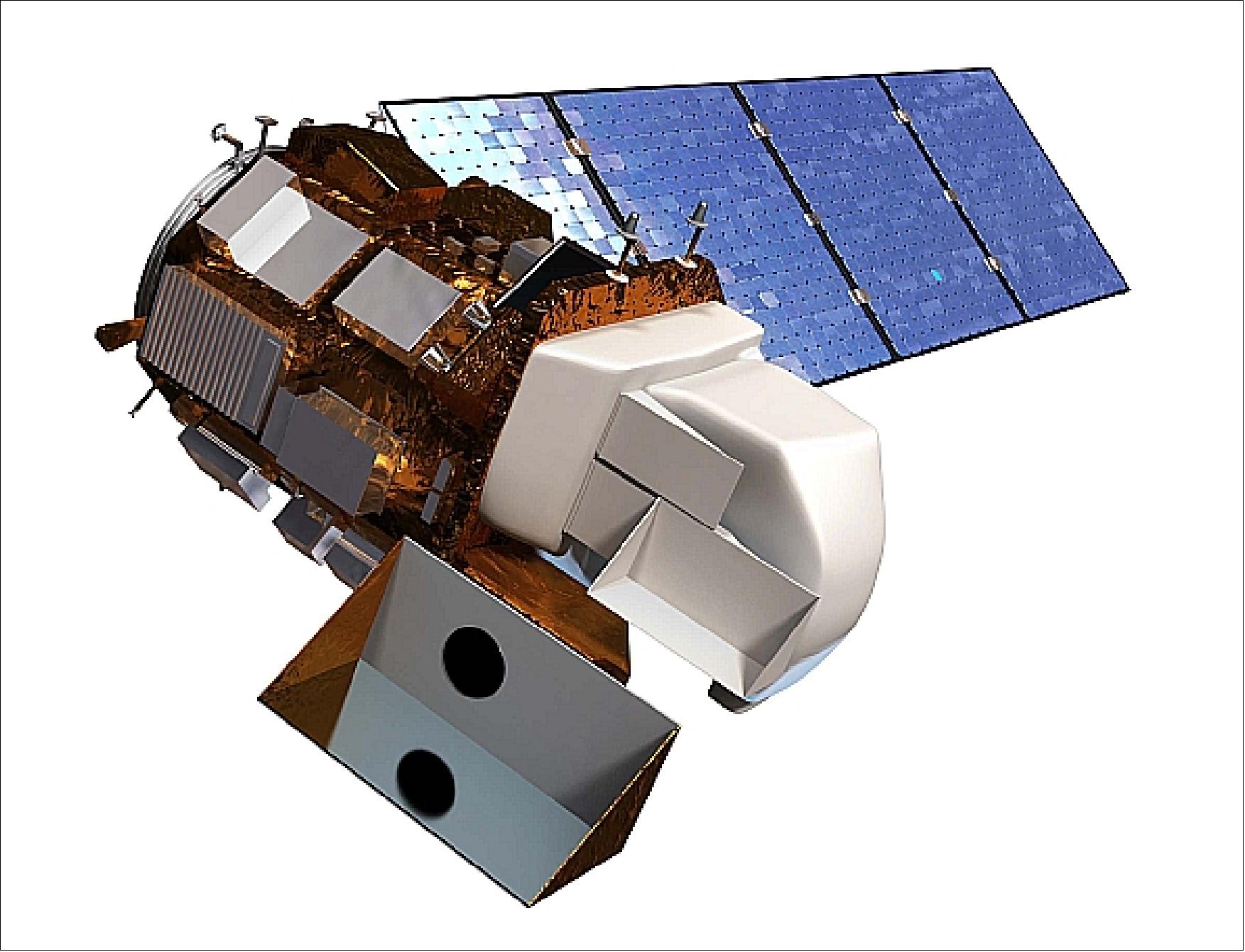
Figure 10: The LDCM spacecraft with both instruments onboard, OLI and TIRS (image credit: USGS) 24)
Launch
The LDCM mission was launched on February 11, 2013 from VAFB, CA. The launch provider was ULA (United Launch Alliance), a joint venture of Lockheed Martin and Boeing; use of the Atlas-V-401 the launch vehicle with a Centaur upper stage. 25) 26)
Note: Initially, the LDCM launch was set for July 2011. However, since this launch date was considered as too optimistic, NASA changed the launch date to the end of 2012. This new launch delay buys some time for an extra sensor with TIR (Thermal Infrared) imaging capabilities.
Orbit: Sun-synchronous near-circular orbit, altitude = 705 km, inclination = 98.2º, period = 99 minutes, repeat coverage = 16 days (233 orbits), the nominal LTDN (Local Time on Descending Node) equator crossing time is at 10:00 hours. The ground tracks will be maintained along heritage WRS-2 paths. At the end of the commissioning period, LDCM is required to be phased about half a period ahead of Landsat 7. 27)
Note: As of February 2020, the previously single large Landsat-8 file has been split into five files, to make the file handling manageable for all parties concerned, in particular for the user community.
• This article covers the Landsat-8 mission and its imagery in the period 2022, in addition to some of the mission milestones.
• Landsat-8 imagery in the period 2021
• Landsat-8 imagery in the period 2020
• Landsat-8 imagery in the period 2019
• Landsat-8 imagery in the period 2018
• Landsat-8 imagery in the period 2017 to June 2013
Mission Status
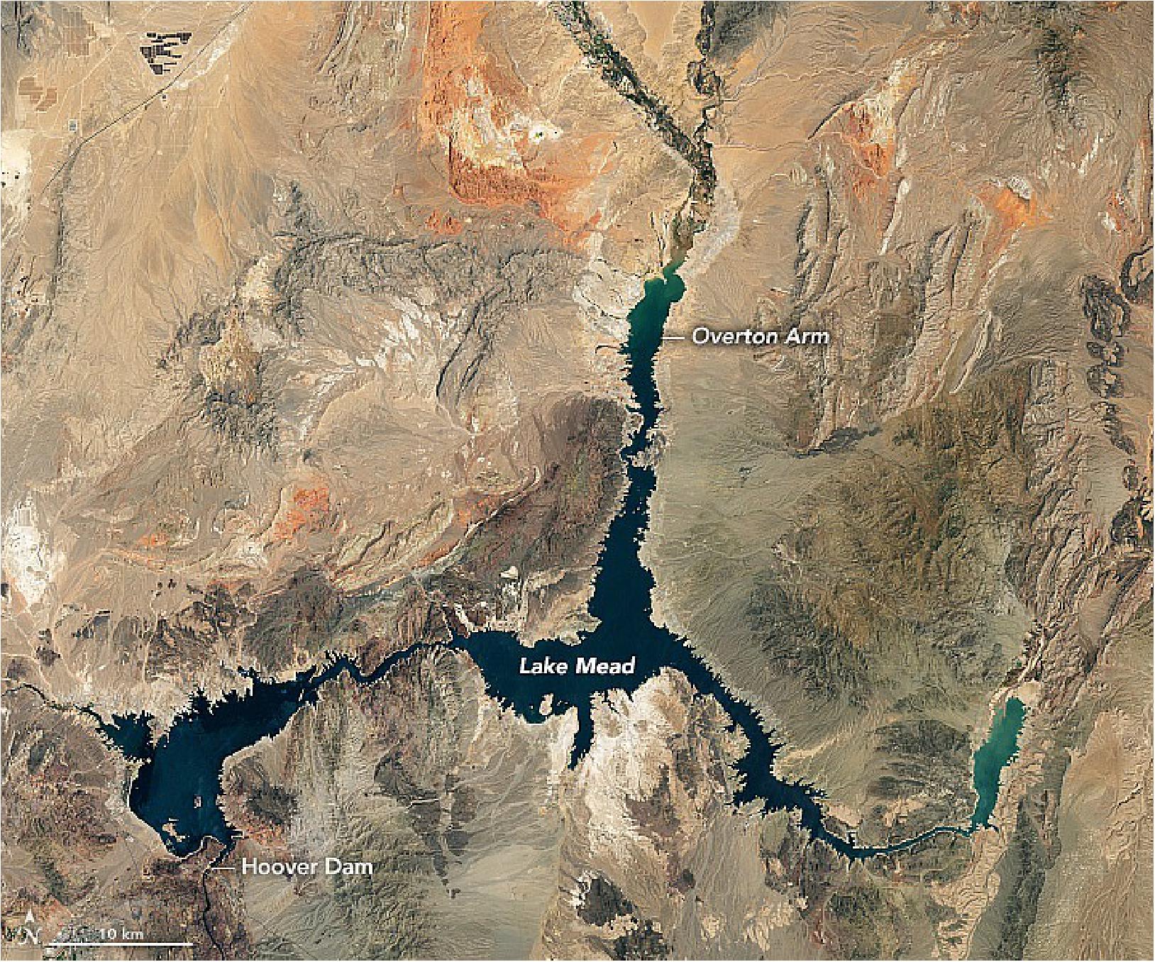
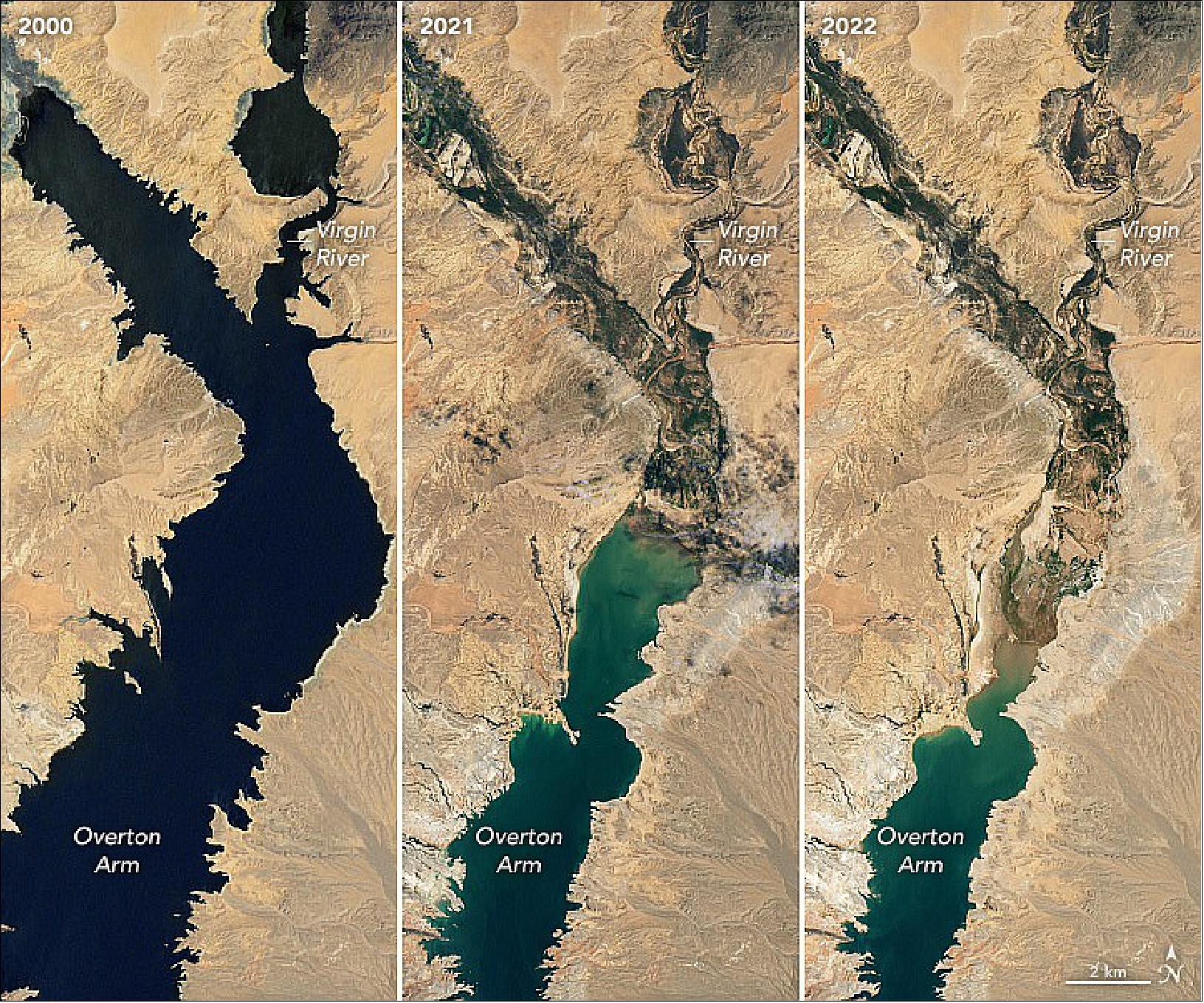
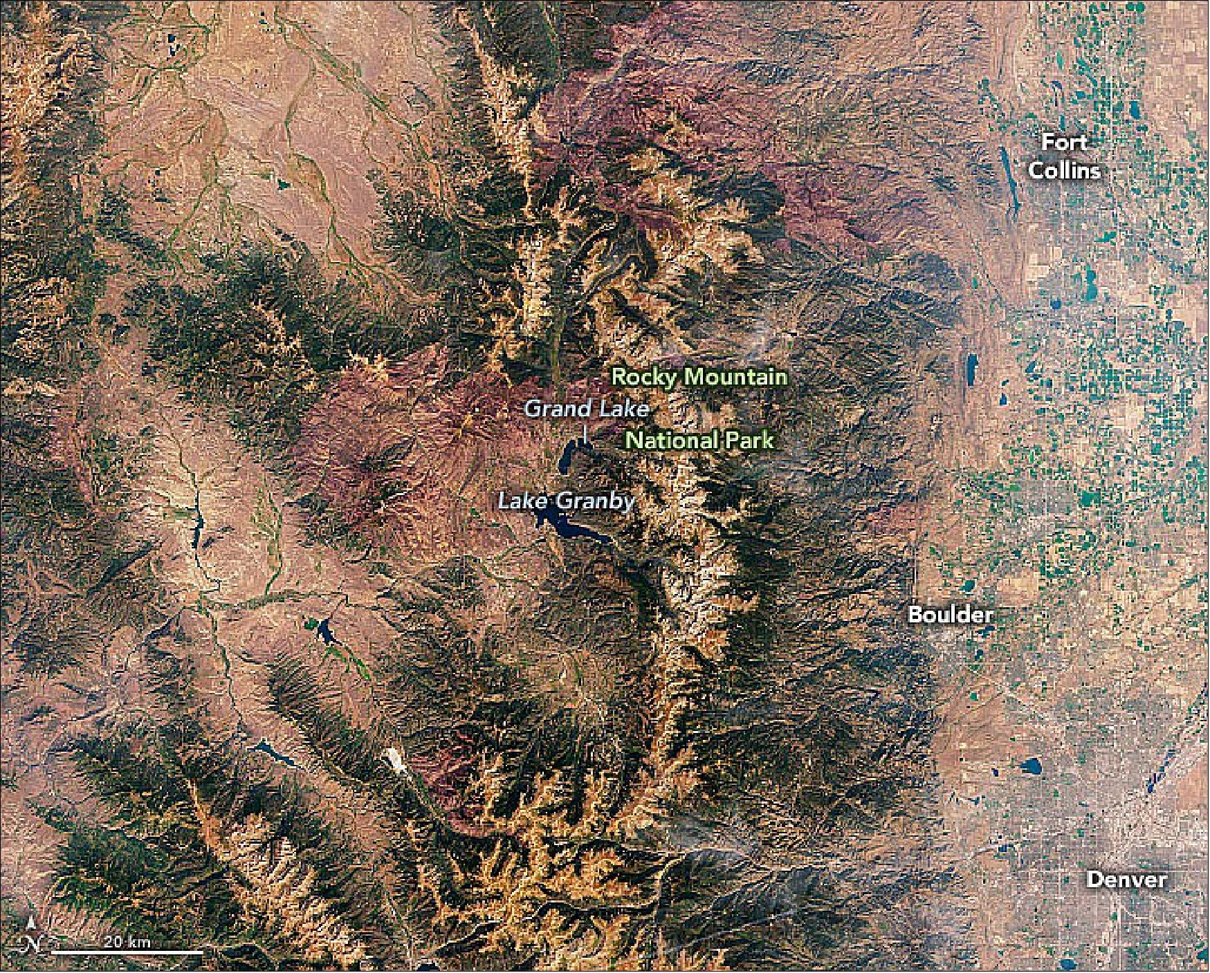
• July 22, 2022: Continuing a 22-year downward trend, water levels in Lake Mead stand at their lowest since April 1937, when the reservoir was still being filled for the first time. As of July 18, 2022, Lake Mead was filled to just 27 percent of capacity. 30) The largest reservoir in the United States supplies water to millions of people across seven states, tribal lands, and northern Mexico. It now also provides a stark illustration of climate change and a long-term drought that may be the worst in the U.S. West in 12 centuries. The low water level comes at time when 74 percent of nine Western states face some level of drought; 35 percent of the area is in extreme or exceptional drought. In Colorado, location of the headwaters of the Colorado River, 83 percent of the state was now in drought, and the snowpack from last winter was below average in many places.
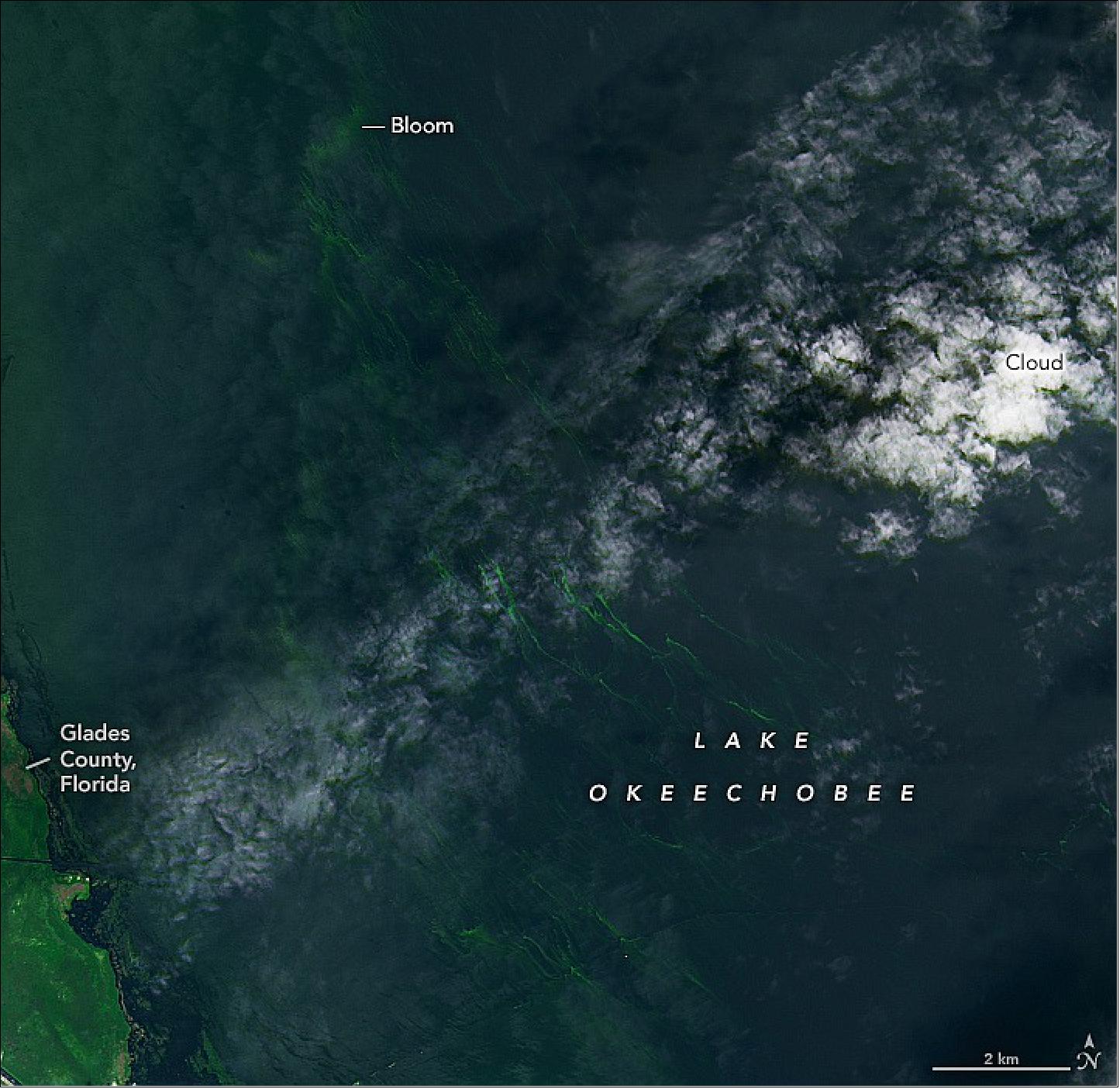
• July 16, 2022: As it has in most recent summers, Lake Okeechobee has been teeming with blue-green algae in 2022. Fueled by warm summer temperatures and abundant nutrients in Florida’s largest freshwater lake, the algae have been blooming since May but significantly increased in abundance through June. 31)
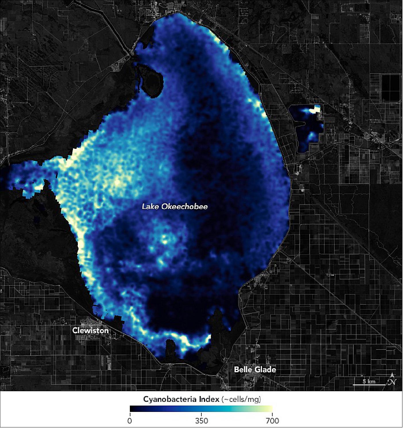
- The Florida Department of Environmental Protection (DEP) reported that 45 percent of the lake was covered with algae or had conditions very conducive to it. The coverage is comparable to levels in July 2021 and 2020, but not as extreme as in 2018, when cyanobacteria blooms covered about 90 percent of the lake. Though popularly called blue-green algae, the formal name for the floating, plant-like organisms is cyanobacteria. These single-celled organisms are among the oldest life forms on Earth, and they rely on photosynthesis to turn sunlight into food. Blue-green algae grow swiftly when nutrients like phosphorus and nitrogen are abundant in still water. They produce a toxin known as microcystin that can sicken people and animals, contaminate drinking water, and force closures of boating and swimming sites. In a 2019 study based on Landsat data, environmental scientists examined 71 large lakes on six continents. They found that the intensity of phytoplankton blooms rose considerably in 48 out of the 71 lakes (68 percent). Most of the increases occurred in the 21st century.
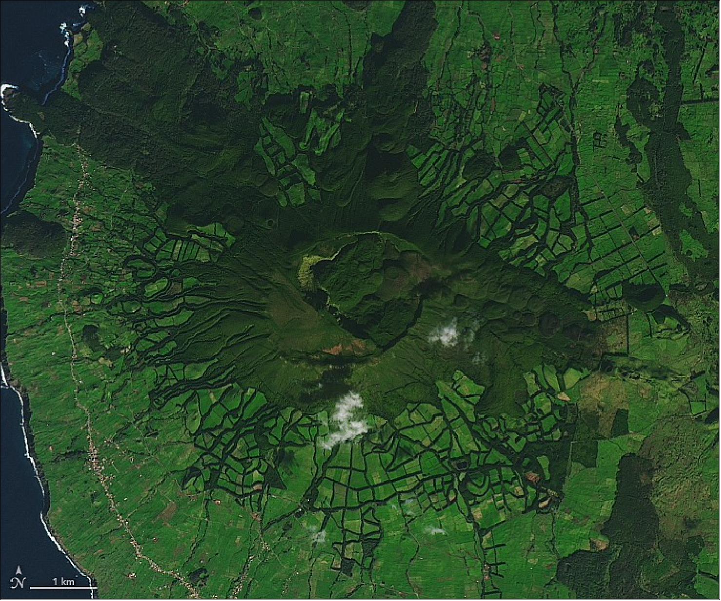
• July 7, 2022: In the eastern mid-Atlantic, 1,800 kilometers west of the Strait of Gibraltar, the Azores archipelago lies at the junction of the North American, Eurasian, and African plates. The volcanically and seismically active island chain began to form about 10 million years ago over a hotspot in Earth’s mantle. Today, this autonomous region of Portugal is a UNESCO Global Geopark. 32)
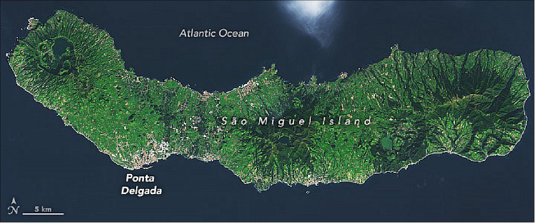
- At 760 km2 (290 square miles), São Miguel is the largest of the nine Azores islands and home to half of its people—most of whom live in Ponta Delgada, the economic capital of the Azores. The island’s highest point is Pico da Vara, which rises to an elevation of 1,080 meters (3,545 feet) above sea level. São Miguel comprises six volcanic zones that formed in the last 3 million to 4 million years. But the island didn’t take on its modern shape until about 50,000 years ago, when an eruption of land-forming lava joined the eastern and western volcanic massifs. The oldest of the six volcanic zones is in the east; the youngest is in the west, where the most recent volcanic activity occurred. Three of the volcanos are still active, though dormant, including Sete Cidades, which last erupted from a submarine vent off the west coast in 1880.
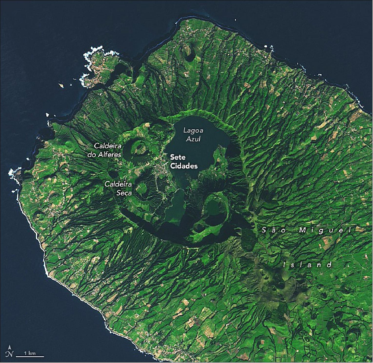
- Sete Cidades Lake is made up of two connected branches: Lagoa Verde (Green Lake) and Lagoa Azul (Blue Lake). Together they cover 4.5 km2 (1.7 square miles). The lake water is high in sodium and chloride due to sea salt spray. The lakes are also prone to eutrophication, or excess nutrients. These phosphorus and nitrogen inputs come from agricultural activities, including livestock. Eutrophication happens most often in the northern part of Green Lake, leading to excess aquatic plant growth and algal blooms. Satellite measurements of the “greenness” of crops, the Normalized Difference Vegetation Index (NDVI), are important for NASA Harvest’s analysis.
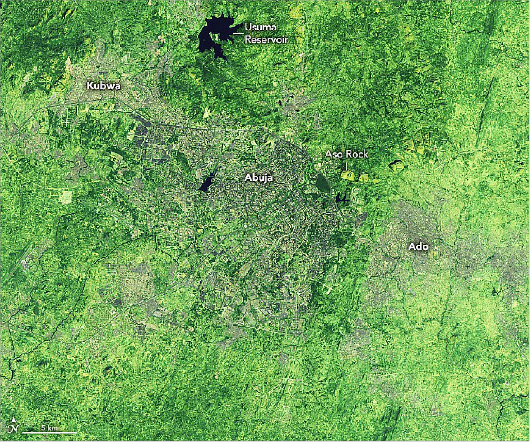
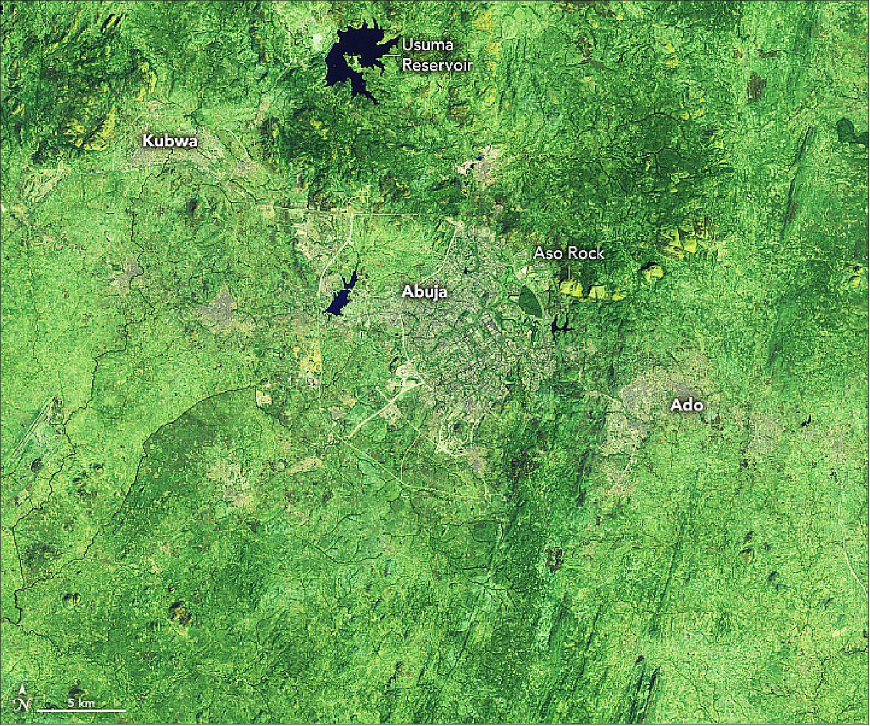
- The city’s master plan called for development to extend outward from Aso Rock in phases, mostly to the southwest. Initially, development proceeded in a somewhat orderly fashion. But one team of researchers that tracked Abuja’s development trends with Landsat data noted that large amounts of unplanned development serving low-income Nigerians began to spring up outside of the planned neighborhoods. The unplanned development was often centered in satellite towns in Abuja’s suburbs, including Ado and Kubwa. The same team found that the percentage of forested land in Abuja Federal Capital Territory has remained at about 10 percent since the 1980s. However, the researchers observed significant losses of forest southeast of the city due to logging and agriculture. The losses have been offset by the establishment of many new forests in parks and preserves throughout the territory.
• June 22, 2022: Lying in the middle of the Atlantic Ocean about 1,400 km (870 miles) off Portugal’s coast, the Azores archipelago is an autonomous region comprised of nine islands and home to almost a quarter million people. The islands are clustered in three groups in a chain spanning 600 km (370 miles) across the Mid-Ocean Ridge. The westernmost island group lies on the North American tectonic plate, while the central and eastern groups lie on the Eurasian plate. 35) The islands of the Azores began to form about 10 million years ago over a mantle hotspot, similar to the formation of the Hawaiian Islands. However, unlike Hawai'i, which lies in the middle of a tectonic plate, the Azores lie on the edge. The North American, Eurasian, and African plates meet to form the Azores triple junction, an uncommon type of plate boundary where three divergent ridges meet. (Most triple junctions involve a subduction zone where plates converge.) The North American and Eurasian plates are moving apart at a rate of 2 to 5 cm (0.75 to 2 inches) per year, an average speed for a spreading center. The Eurasian and African plates, however, are diverging at a hyperslow rate of 2 to 4 mm (0.08 to 0.16 inches) per year along the 550-km (340-mile) Terceira Rift.
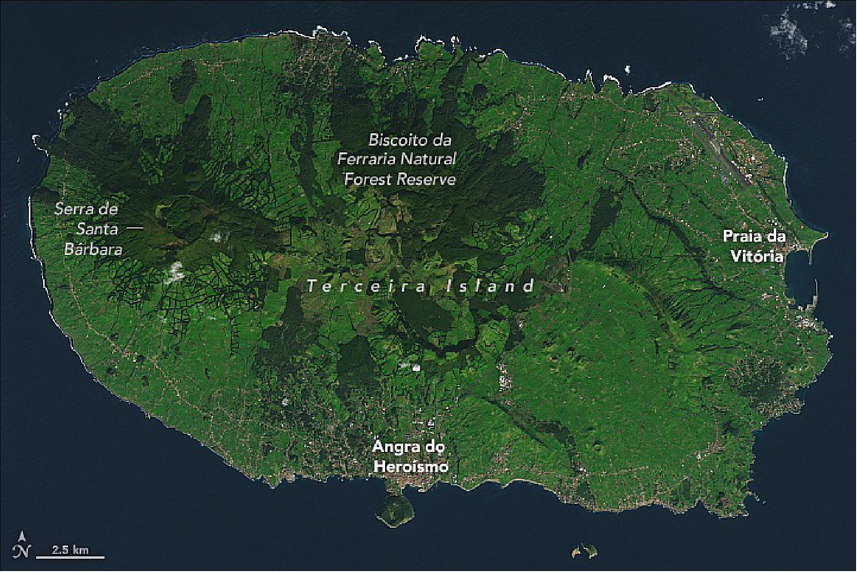
- The flanks of the volcano are covered by agricultural fields and pastures. The island’s most recent volcanic activity occurred underwater on the Serreta Volcanic Ridge, which lies about 10 kilometers (6 miles) west of the island. That eruption started in December 1998 and continued through March 2000. During this eruption, a submarine plume emitted basalt balloons. These hot blobs of basaltic lava contain volcanic gases that expand, causing the lava balls to inflate and float to the surface. Once the gas dissipates and the lava is quenched by seawater, the newly formed igneous rocks sink back to the seafloor.
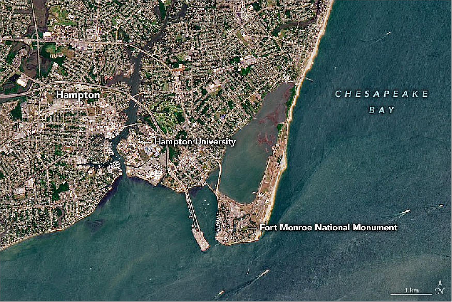
• June 19, 2022: About 35 million years ago, an asteroid or comet smashed into the continental shelf near what is now the mouth of Chesapeake Bay. Among the areas in the blast zone was Old Point Comfort, the southernmost spit of land on the Virginia Peninsula. That same piece of land was later the site of a historical collision that reverberates to this day. 36) The rate of sea level rise has accelerated to roughly one inch every four years due to ongoing subsidence of the land, warming waters, and other factors related to climate change. Sea level rise projections from the Interagency Sea Level Rise Scenario Tool (published by NASA’s Sea Level Change Team) indicate that Sewell’s Point in Hampton Roads could experience between 0.69 and 2.2 meters (2 and 7 feet) of sea level rise by 2100.
• June 11, 2022: Bezymianny Volcano on the Kamchatka Peninsula in Russia's Far East rises to a summit elevation of 2,882 meters (9,455 feet). The name, which translates to “no name,” was likely bestowed because the stratovolcano had been quiet for a thousand years at the time it was named. Until late 1955, when it awakened with a cataclysmic eruption, the volcano was considered extinct. Bezymianny has been erupting intermittently ever since. 37) The 1955–1956 eruption was very similar to the 1980 eruption of Mount St. Helens, with a lateral flank explosion and summit collapse producing a mile-wide horseshoe-shaped crater. Continuing volcanic activity, including the resurgence of a lava dome and pyroclastic flows, has since filled in the 1956 crater.
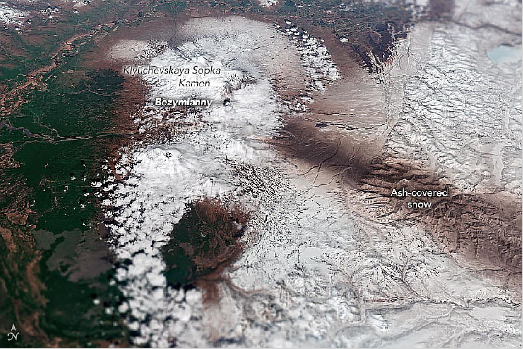
- On May 28, 2022, Bezymianny erupted again with a strong explosion and large ash plume recorded by observers at the Kamchatka Volcanological Station. The ejected ash ultimately reached an altitude of 15 km (9.3 miles) and traveled east-southeast for more than 1,600 km (1,000 miles). As the plume drifted over the peninsula toward the Pacific Ocean, it deposited a layer of ash on the snow-covered ground. The ash cloud prompted a red-level aviation alert before being lowered to orange; the second highest alert on a four-level, colour-coded scale. The Kamchatka Peninsula is home to more than 300 volcanoes, 20 of which are active, making it one of the most volcanically and geothermally active regions in the world. The peninsula rides on the Okhotsk Plate, with the Pacific Plate diving under it at a rate of 8 to 10 centimeters per year. Magma generated by the descent of the Pacific Plate into the submarine Kuril-Kamchatka Trench has given rise to three volcanic arcs, or arcuate ranges of volcanoes, on the peninsula above.
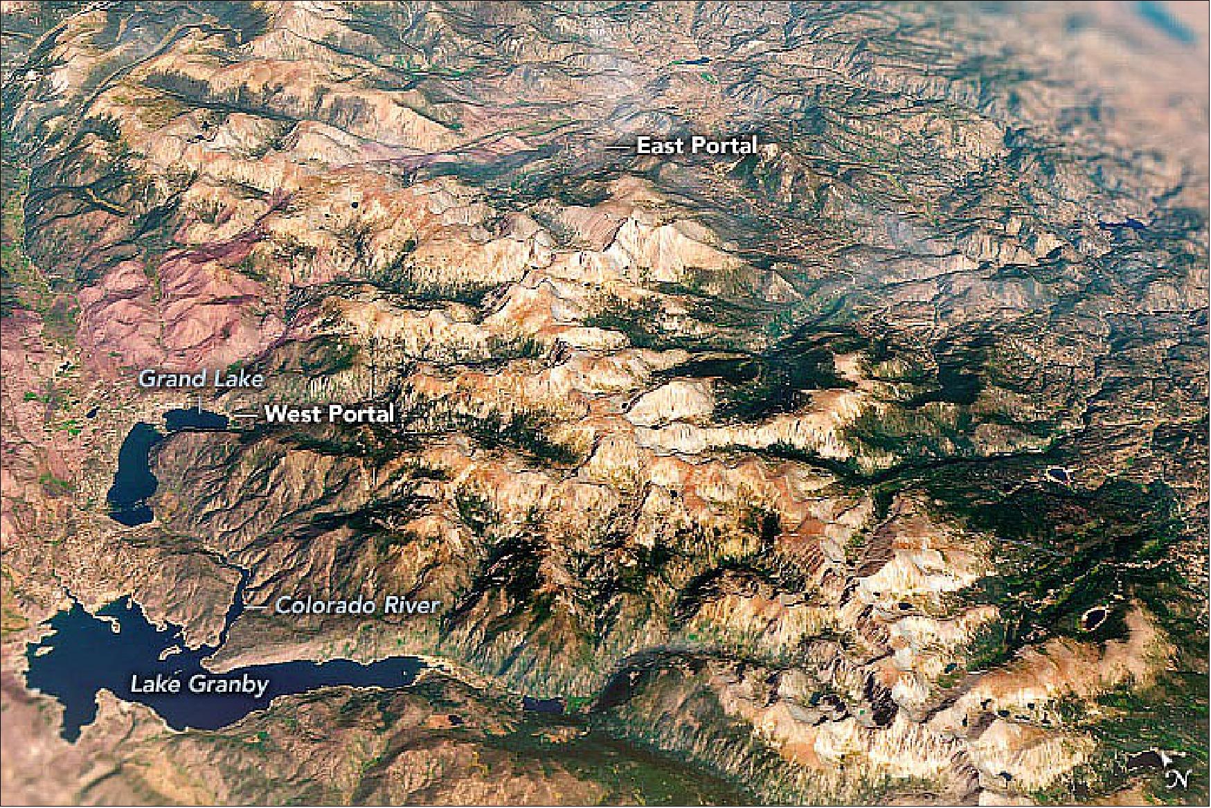
• June 9, 2022: A 20-kilometer-long tunnel under Rocky Mountain National Park diverts water from the Western Slope of the Rockies to Colorado’s Front Range and eastern plains. 38) The Western Slope receives 80 percent of the state’s precipitation, as weather systems rising to cross the continental divide shed their loads of rain and snow before moving east. Water that falls to the west of the divide drains toward the Pacific Ocean, while water that falls to the east runs toward the Gulf of Mexico and Atlantic. The Colorado-Big Thompson project delivers 200,000 acre-feet of water a year to northeastern Colorado, quenching the thirst of one million residents and irrigating more than 600,000 acres of farmland. Although the diversion project was initially built to irrigate farms and fields, it now also supplies water for cities and towns, industry, hydropower generation, recreation, and fish and wildlife. In Colorado, where more than 80 percent of the people live where only 20 percent of the precipitation falls, such transbasin water diversions have become a part of life.
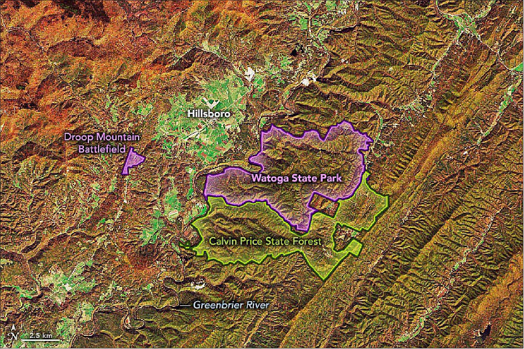
• June 6, 2022: Amid the network of artificial lights lights that span our planet like a game of connect-the-dots, darkness is a precious commodity. There are places, however, where the terrain and distance from cities help keep light pollution to a minimum. Watoga State Park in eastern West Virginia is one such place. 39) Watoga and the nearby Calvin Price State Forest and Droop Mountain Battlefield State Park combine to span a total of 31 square miles (80 km2) of Pocahontas County. Located in the highlands of the Allegheny Mountains, the parks are relatively remote, far from the glow of major cities that light up much of the eastern United States. Only a handful of small towns and farms dot the otherwise heavily forested landscape.Recent changes have made the parks even darker than just a few years ago.
- The Watoga State Park Foundation obtained funding that allowed them to replace existing lights throughout the park with new fixtures that aim downward and use bulbs that cause less light pollution. In addition, volunteer astronomers tracked the quality of nighttime darkness over the span of a year, and the park held several events to educate the public about dark skies. The efforts culminated in all three parks receiving official status as “dark sky parks” in October 2021. They were the state’s first parks to receive the designation from the International Dark-Sky Association While dark skies are favored by stargazers, they are also important for the local ecology. The park is home to the rare “synchronous” firefly. It’s the timing of their flashes, made in rhythmic, synchronised intervals, that sets their mating display apart from other fireflies. Watoga State Park is one of a handful of public locations in the United States where people can view the display. The park’s protection from light pollution should also benefit the fireflies, which are sensitive to light.

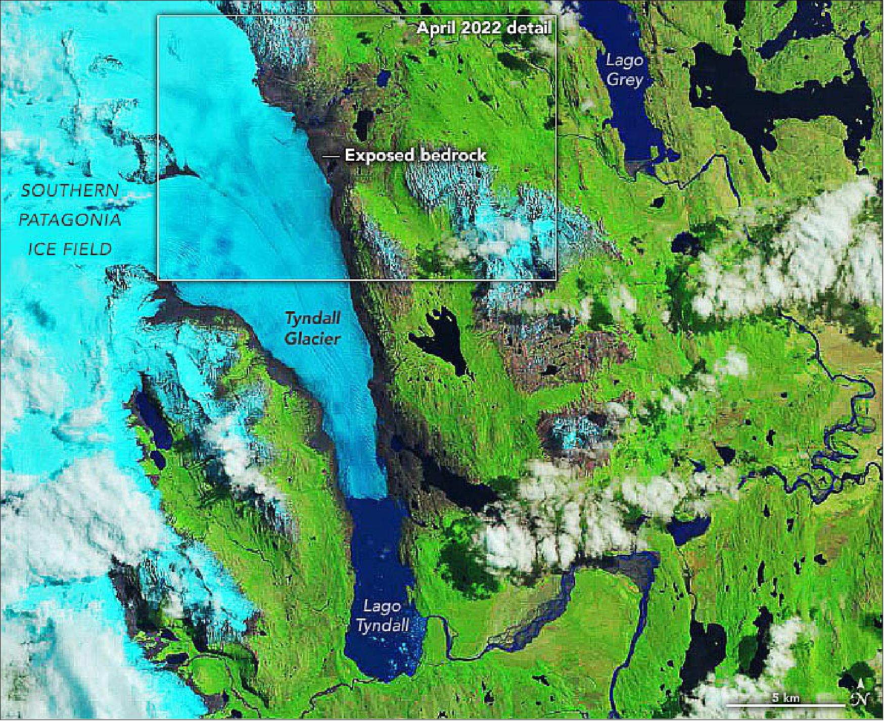
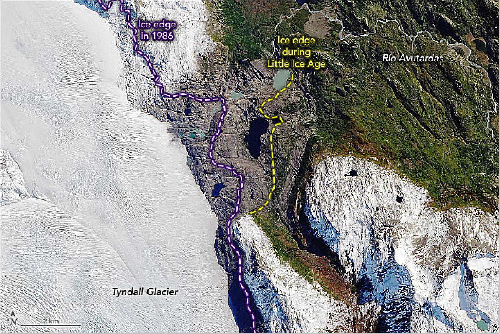
• June 3, 2022: As glaciers have melted in our warming world, they have exposed pieces of the past, from Stone Age artifacts to wartime relics. But the retreating Tyndall Glacier in Chile has uncovered something much older: a prehistoric graveyard of ichthyosaurs. 40) Ichthyosaurs were marine reptiles, or “fish lizards,” that resembled modern-day porpoises. They swam in the oceans between 250 and 90 million years ago, around the same time that dinosaurs walked on land and pterosaurs soared in the air. The creatures are now extinct, but their fossils continue to inform scientists about the species and how they evolved. So far, paleontologists have found 76 ichthyosaurs in the bedrock adjacent to Tyndall Glacier in the Southern Patagonia Ice Field. Some of the fossils were uncovered during an expedition to the site in March and April 2022, when scientists visited to extract “Fiona,” a complete fossilised skeleton of a 4-meter-long female with several embryos, between 129 and 139 million years old. Just a few decades ago, paleontologists would have likely missed some of these discoveries. Camilo Rada, a glaciologist at University of Magallanes, estimated from photographs that Fiona has been uncovered since at least 1965. “But other ichthyosaur fossils in the area were uncovered much earlier, others much more recently, and in all likelihood, some are becoming uncovered as we speak,” Rada said.
• May 31,2022: The chain of hundreds of low-lying islands, also called cays or keys, that extend from southern Florida are relics of a time when global sea levels were higher than today. About 125,000 years ago, during a warm interglacial period, water covered the area. 41)
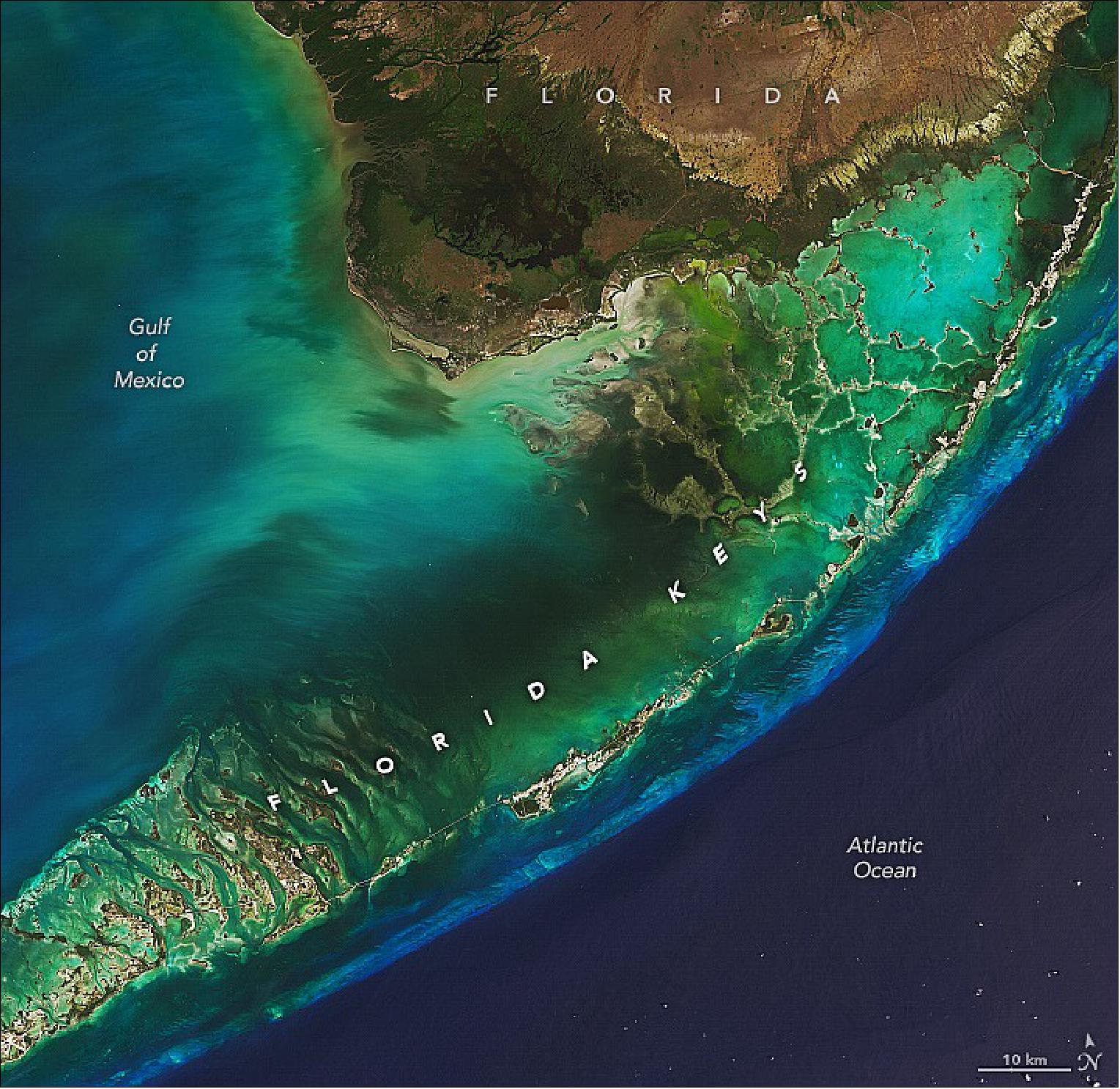
- However, the sea was shallow enough that big communities of coral flourished just below the surface and built up reefs. The Florida Keys formed as coral reefs and sand bars fossilised during an ice age when sea levels dropped. Today, the Keys' sedimentary rocks reflect these ancient formations. Many of the Florida Keys fall within the boundaries of national parks. Biscayne National Park includes several of the northernmost keys. Most of those within Florida Bay are part of Everglades National Park. The westernmost keys fall within Dry Tortugas National Park. The Florida Keys National Marine Sanctuary protects many of the keys as well. More than 80,000 people live on 30 populated islands, and several million people visit the Florida Keys each year. Still, some parts of Big Pine Key and several other islands retain patches of pine rockland, an unusual ecosystem found exclusively in southern Florida. In these areas, scattered slash pine soars over an understory of palms, palmettos, berries, grasses, and several types of herbaceous plants. While falling sea levels brought the Florida Keys into existence, rising seas now pose a threat to their long-term existence. Sea level rise projections from the Interagency Sea Level Rise Scenario Tool (published by NASA’s Sea Level Change Team) indicate that Key West could experience between 0.45 and 2.16 meters (1 and 7 feet) of sea level rise by 2100.
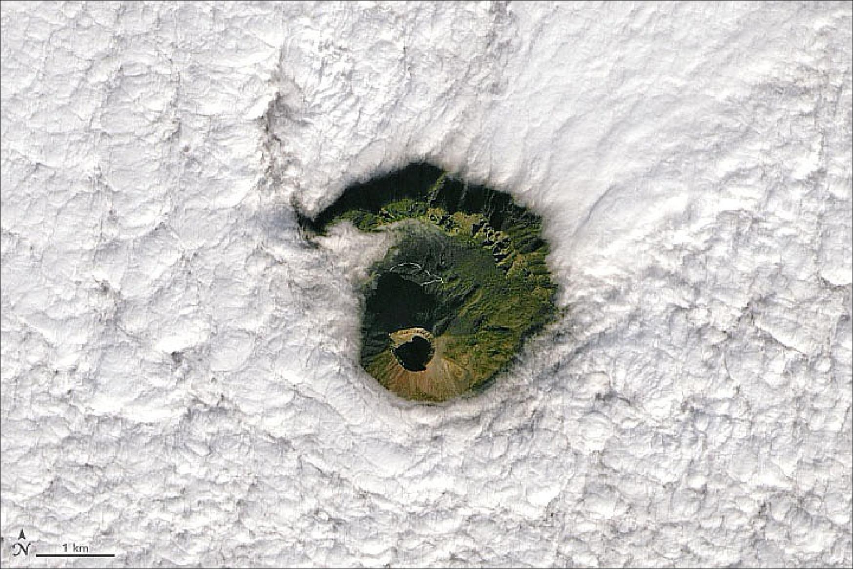
• May 30, 2022: The island of Manam, in the Bismarck Sea off the northeastern coast of Papua New Guinea, is one of the most active volcanoes in the South Pacific. In May 2022, the Darwin Volcanic Ash Advisory Centre issued several aviation alerts for ash plumes rising from Manam. On May 17–19, ash plumes reached altitudes up to 2.4 km (1.5 miles) above sea level and drifted northwest and west. 42) Manam is a stratovolcano, a type known for explosive eruptions that create steep-sided cones. Frequent mild-to-moderate explosive eruptions have been recorded here since 1616. They most often produces ash plumes, but occasional larger eruptions have produced lava and pyroclastic flows that reached the coast.
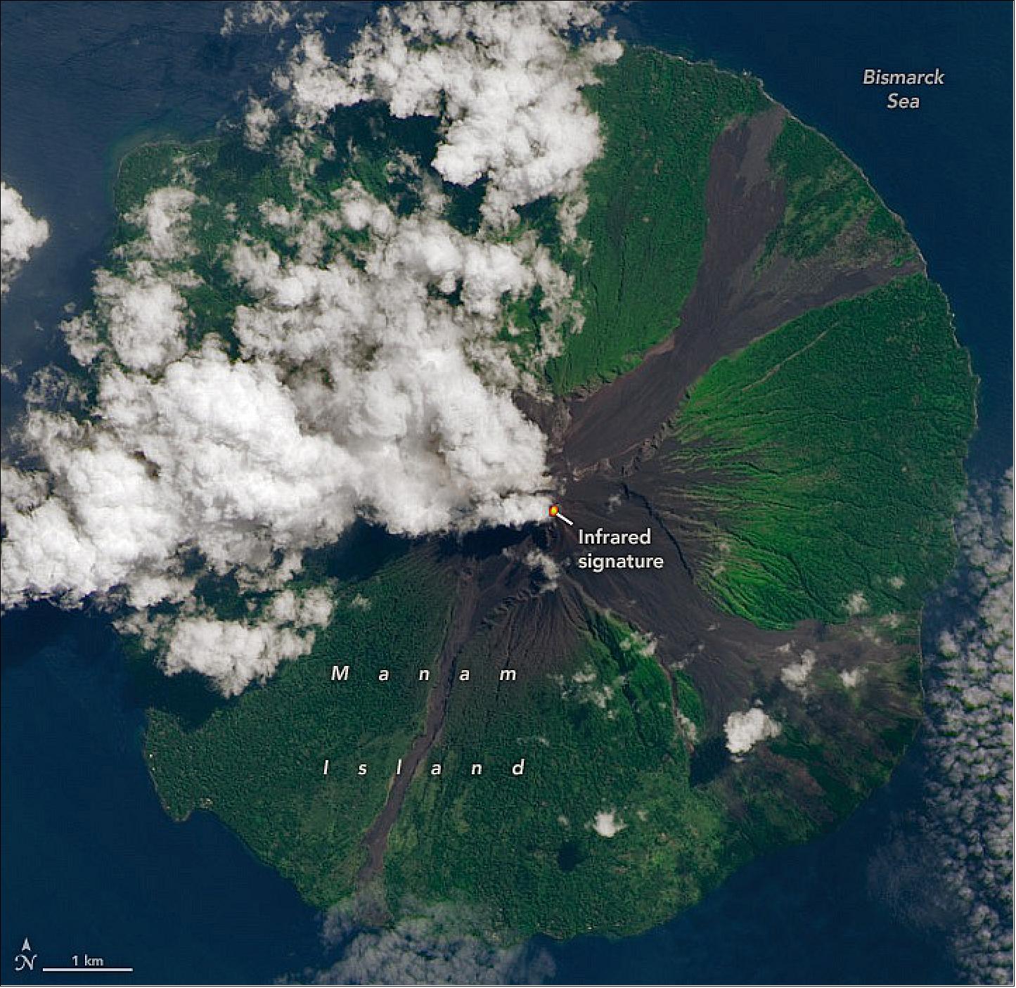
- An October 2021 eruption emitted an incandescent plume and ejected an ash cloud to a height of 15.2 kilometers (9.4 miles). Intermittent ash plume eruptions continued in late 2021 and into 2022. In early March 2022, researchers from the Rabaul Volcanological Observatory reported a small pyroclastic flow descending Manam’s flank. The eruption was accompanied by ash emissions. Four valleys radiate from the classic conical peak of this stratovolcano, which rises to an elevation of 1,800 meters (5,900 feet) above sea level. Three of the valleys, locally called avalanche valleys, are visible in the image. The valleys have channeled many of the previous lava and pyroclastic flows, some of which enter the sea. However, some eruptions have jumped out of the valleys and reached populated areas on the lower flanks of the volcano. Most of Manam’s 9,000 residents were evacuated during a major eruption in 2004, but many people have since returned. The 2005 eruption sent a large cloud of sulfur dioxide drifting west over the island of New Guinea. Papua New Guinea is home to 14 active and 22 dormant volcanoes that present a risk to an estimated 250,000 people. Of those, Manam is one of six that scientists have categorised as high-risk. The island has also been identified as one of several volcanoes where an eruption or flank collapse could possibly produce a tsunami.
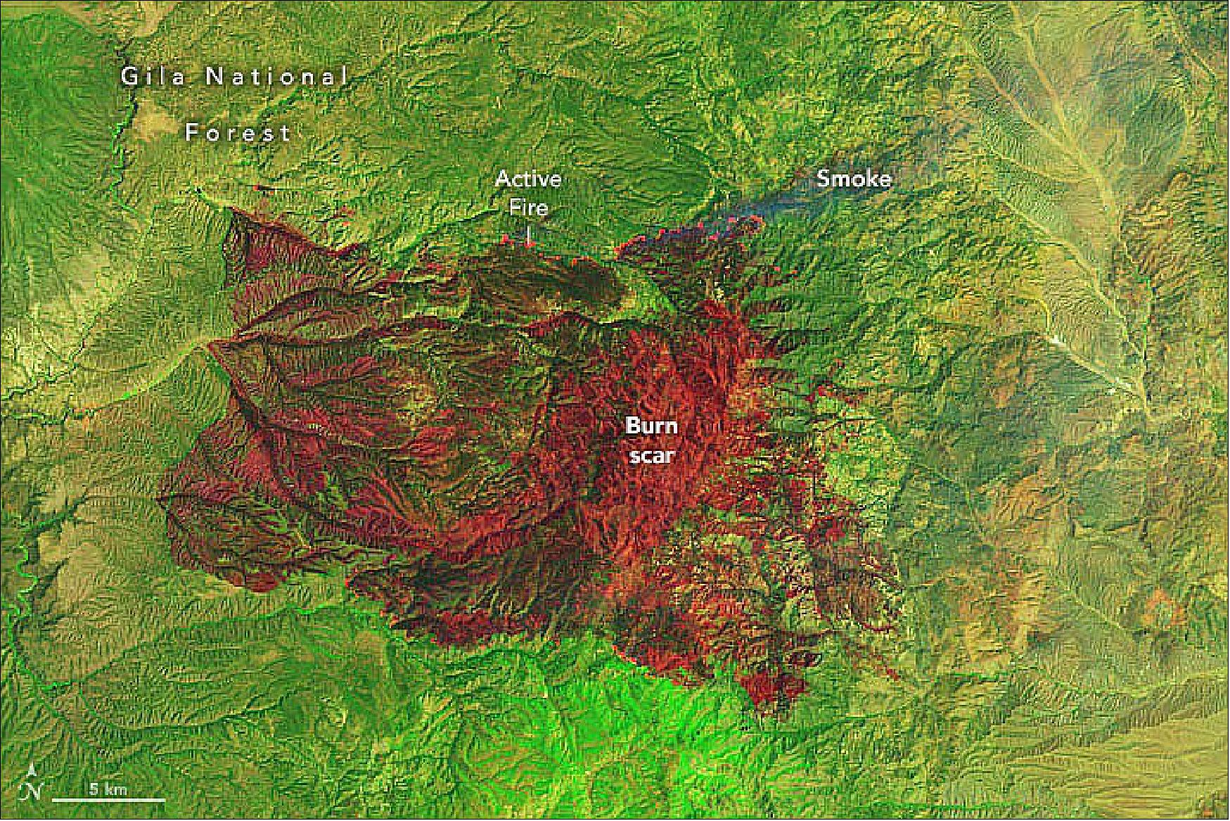
• May 24, 2022: A new wildfire erupted on May 13, 2022, in the Gila National Forest in southwest New Mexico. The state has seen more than half a million acres burned this year in early season wildland fires, and forecasters predicted conditions could worsen through the end of the month. 43) The Black fire began burning in the Aldo Leopold Wilderness Area in the Black Range, about 30 miles northwest of Truth or Consequences, New Mexico. On May 16, the fire blew up, tripling in size from 18,000 acres to more than 56,000 acres. A blow-up is a sudden increase in fire intensity or rate of spread. The blow-up of the Black fire on May 16 produced a small pyrocumulonimbus cloud as the fire ran east and crossed the Continental Divide. As of May 22, the Black fire had burned more than 130,000 acres, becoming the second-largest fire burning in the state. The perimeter was 8 percent contained, with more than 600 firefighters working the blaze.
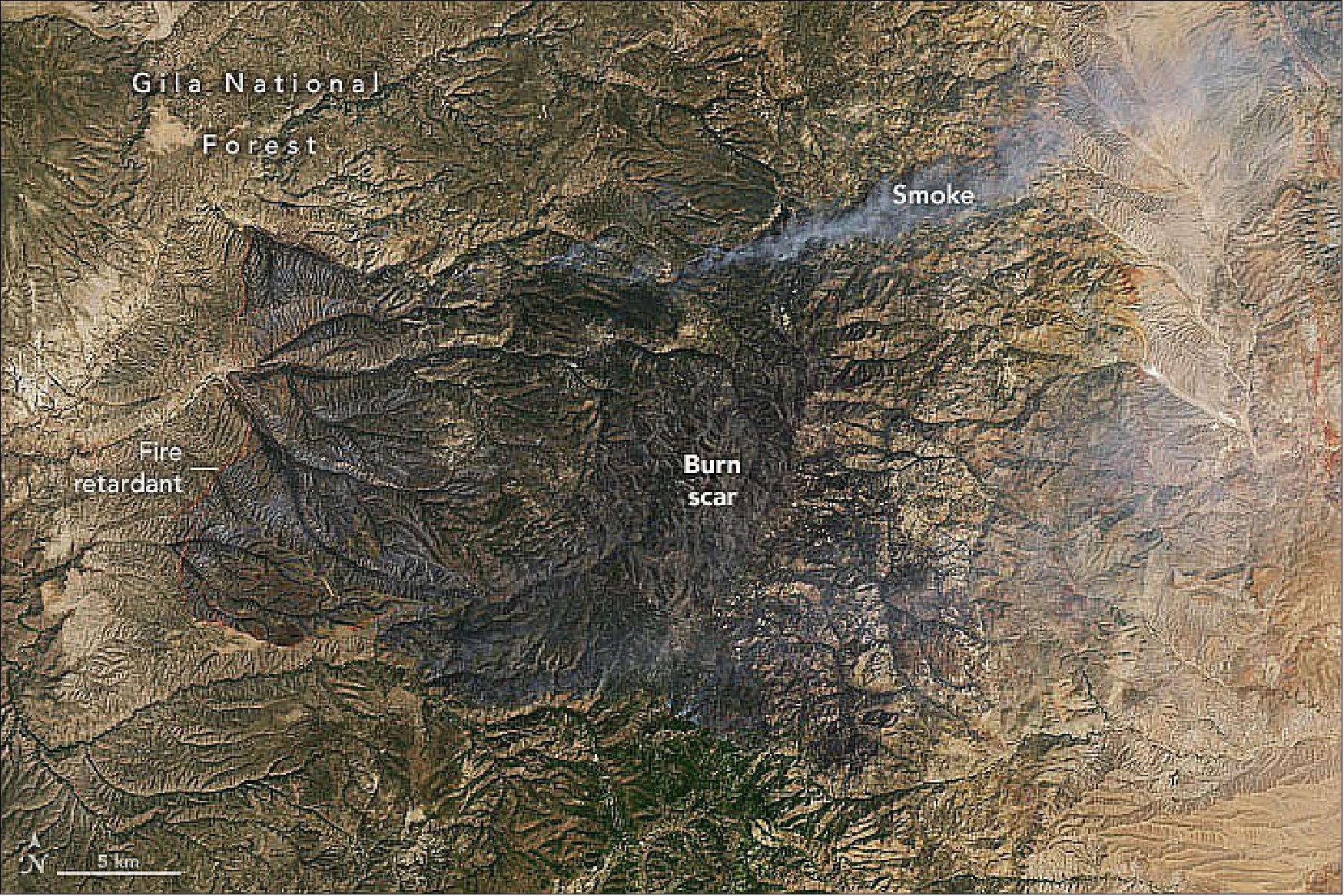
- The Black fire is one of several large uncontained fires burning in New Mexico, including the Calf Canyon-Hermits Peak Fire. As of May 23, 2022, that fire had exceeded 300,000 acres, the largest in state history, and was 40 percent contained. New Mexico has had more than 300 fires so far in 2022, burning more than 580,000 acres, according to the National Interagency Fire Center (NIFC). That is nearly five times as much acreage as was burned in all of 2021.
• May 16, 2022: The surf break known as “Freight Trains” rips across Mā`alaea Bay on Maui’s southern shore. However, surfers suggest that the substantial, surfable break here is relatively rare. Conditions need to be just right: namely, large waves must approach the bay from the perfect south or southeasterly direction. The large waves, or swells, are typically generated in the southern hemisphere during winter, when large storms brew in the southern Pacific Ocean. The waves can travel thousands of miles, crossing the equator and eventually reaching Maui’s southern shore, where it is summer. But the waves can lose energy along the way as they encounter numerous island chains in the South Pacific. 44)
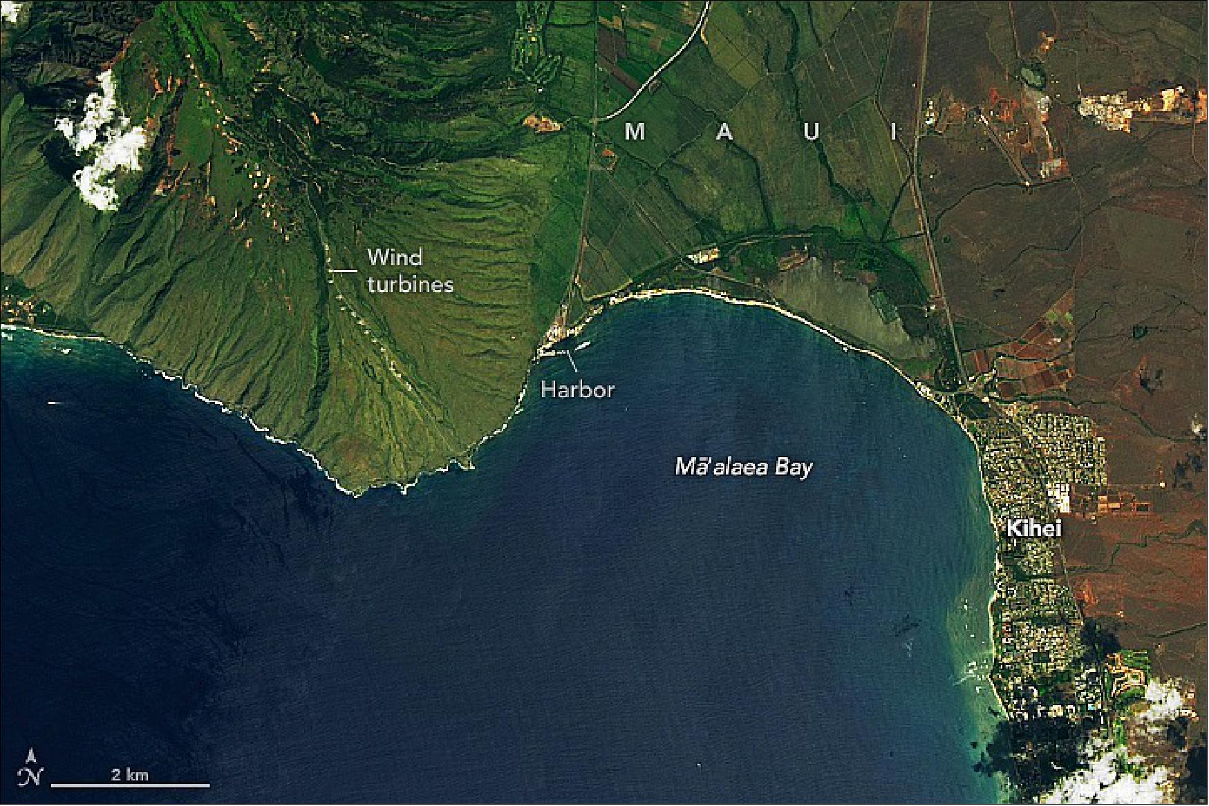
- The strength of offshore winds also matters. Gentle offshore winds support the wave front, helping create the smooth, steep face that surfers seek. But offshore winds that are too strong can prevent a wave from breaking at all. In Mā`alaea, located on the island’s leeward side, strong trade winds from the north are accelerated as the air is forced between the peaks of Mauna Kahālāwai (west) and Haleakalā (east). (Notice the wind turbines in the image above, poised to take advantage of this so-called Venturi effect.)
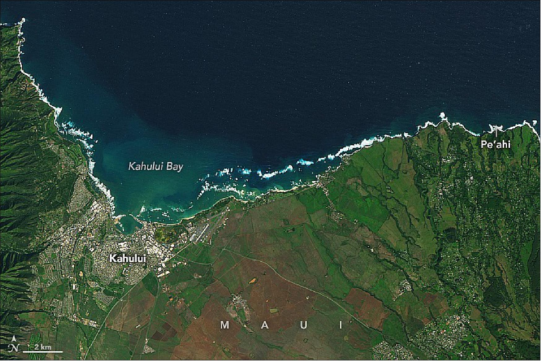
- On the occasions when waves in Mā`alaea Bay do break, they do so with crushing speed like a freight train. The speed is mostly to do with the dramatic transition of the seafloor from deep water to shallows. Strong currents in the bay, possibly enhanced by the harbor, can also make the wave break faster. When waves are ripping in Mā`alaea Bay, conditions are typically quiet off the island’s northern shore—that is, until winter, when storms are brewing in the North Pacific. Winter weather systems in the basin generate the swell that marches toward Maui’s northern shore. Unimpeded by other island chains, they retain more energy during their shorter journey and produce the island’s famously large winter waves.
• May 07, 2022: Ha Long Bay covers about 1,500 km2 (600 square miles) along the northeastern coast of Vietnam and holds more than 1,600 islands. The mountainous limestone islands, the tallest of which tower up to 400 meters (1,300 feet) above the water, are some of the world’s most visible and famous examples of karst features. 45) Karst landscapes form in humid environments with highly soluble and fractured carbonate or evaporate rocks, like limestone or gypsum. These landscapes have distinctive features such as sinking streams, sinkholes, caves, springs, and fluted rock outcrops. Vietnam’s ideal conditions, 24°C temperature, 2,300 mm rainfall, and 90 percent humidity, support karst formations that cover 18 percent of the country, mainly in the north and central areas.
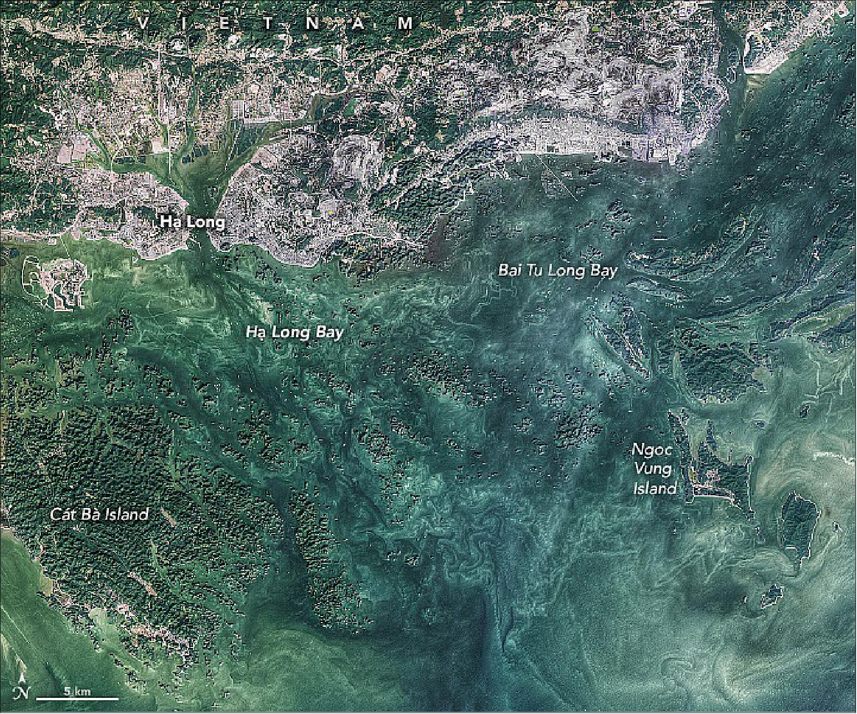
- Ha Long Bay and Bai Tu Long Bay are known for their striking karst features, including caves and conical peaks. Cát Bà Island is famous for its caves and national park. The limestone here formed 390–260 million years ago and was uplifted 40 million years ago, through faulting and plate tectonic activity, shaping the islands through erosion. Karst erosion creates fertile soils that support rich biodiversity, including species unique to Vietnam. The bays are also linked to the legend of the "descending dragon," where dragons formed the islands. Most of the islands in Ha Long Bay, which was named a UNESCO World Heritage site in 1994, are uninhabited and unaffected by humans. Elsewhere, however, karst ecosystems are vulnerable to degradation from mining for cement and other human threats.
• May 05, 2022: Levels of methane in Earth’s atmosphere are soaring. In April 2022, NOAA reported that concentrations of the potent heat-trapping greenhouse gas averaged 1,895.7 parts per billion (ppb) over the past year, a new record. The 17 ppb increase in 2021 was the largest recorded since systematic measurements began in 1983. That followed a 15 ppb increase in 2020. 46)
- Several activities and processes, some natural, some human-caused, affect methane levels. The list includes fossil fuel production, agriculture, fire activity, precipitation, and the presence of methane-scrubbing chemicals (hydroxyl radicals) in the atmosphere. But the global network of monitoring stations only offers a measure of methane that has dispersed throughout the atmosphere; it does not show where the methane is coming from or what specific activities have pushed levels so high. Methane is released from wetlands by armies of anaerobic bacteria that thrive in waterlogged soils and help break down decomposing vegetation. Recently, a growing body of research indicates that certain types of trees found in wetland areas, both living and dead, may also move methane from waterlogged soils into the air or produce the gas directly.
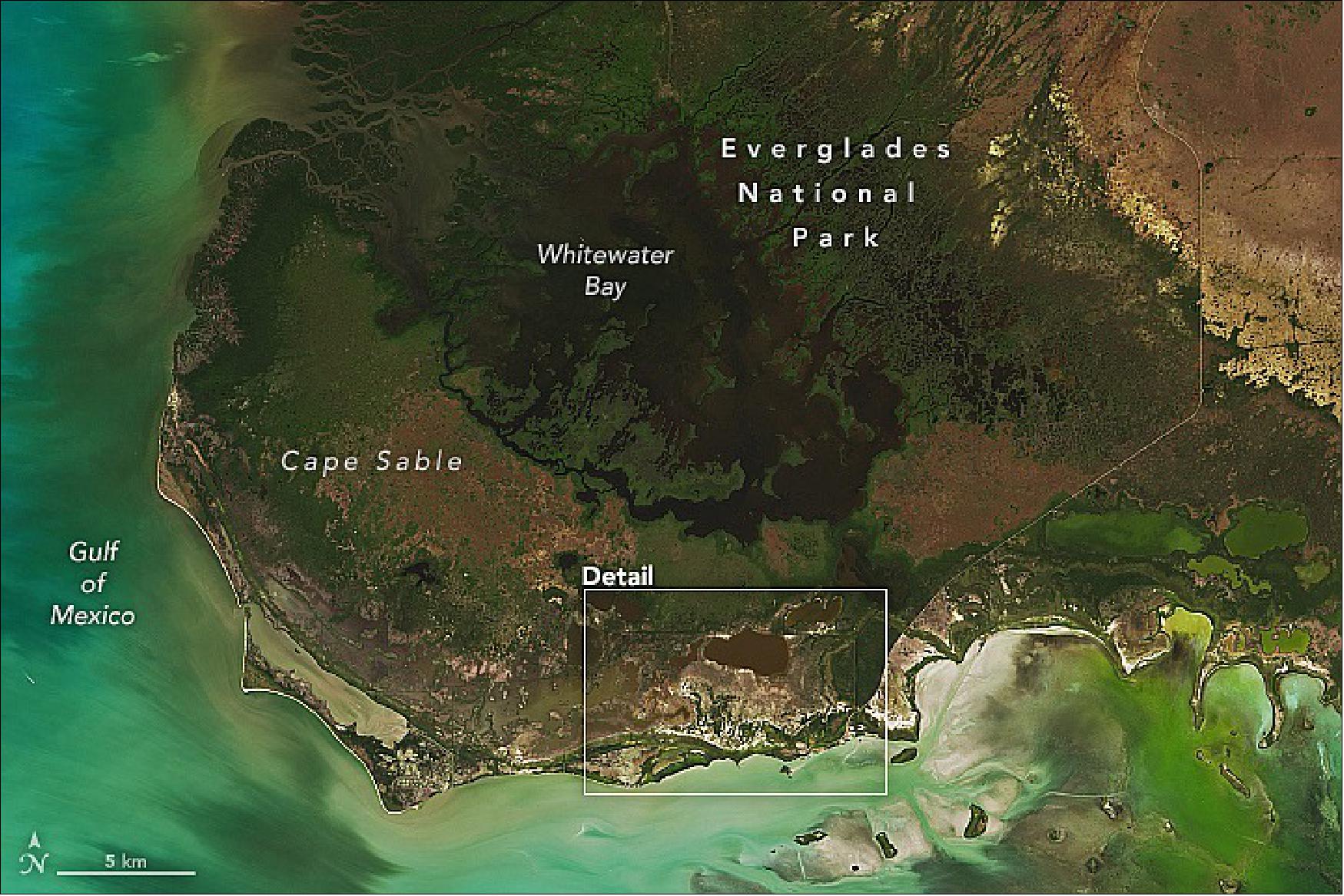
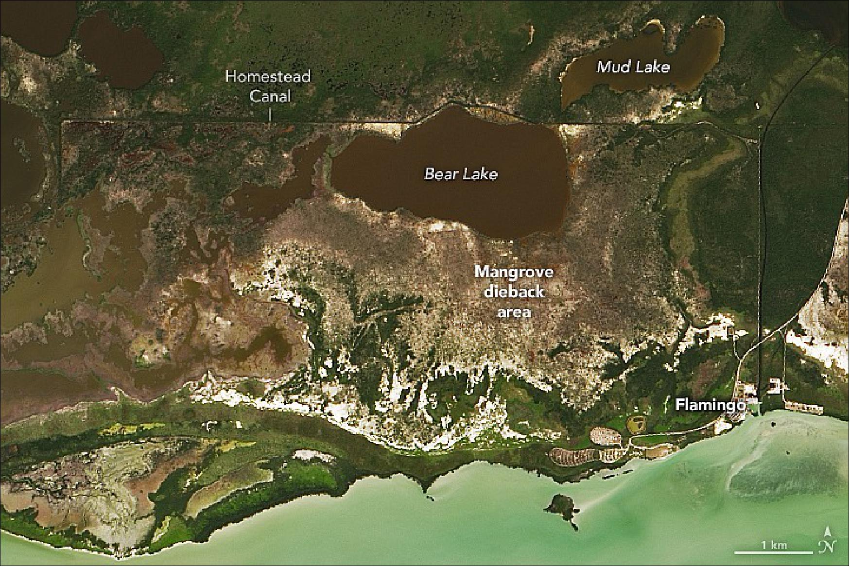
- Mangroves are known for being particularly productive and good at storing large amounts of carbon in the soil around them—perhaps as much as five times more than upland tropical forests. The field campaign, called Blue Carbon Prototype Products for Mangrove Methane and Carbon Dioxide Fluxes (BLUEFLUX), was designed to measure the methane and carbon dioxide changes at key wetlands around the Caribbean. Field teams took samples from the ground, while NASA’s Carbon Airborne Flux Experiment (CARAFE) aircraft measured methane emissions from the same locations from above. The broader goal of the campaign is to link ground and aerial data with satellite observations using machine learning and artificial intelligence algorithms in order to produce a daily methane flux dataset for the Caribbean region.
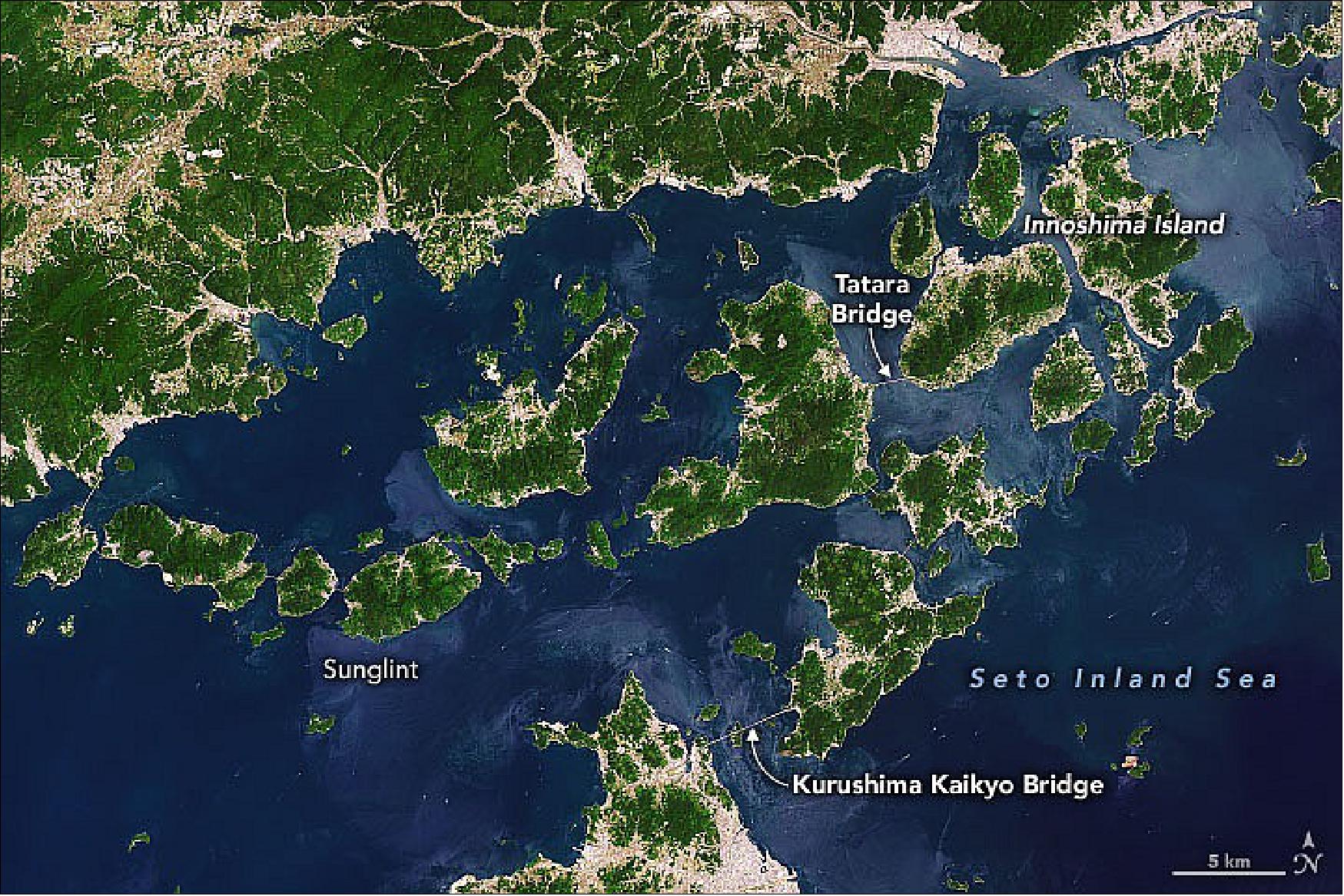
• April 30, 2022: Whirlpools and other complex currents routinely roil Japan’s Seto Inland Sea. Strong tidal currents send water churning through a maze of channels and narrow straits surrounding thousands of islands in the shallow sea. The islands of the Geiyo archipelago are among them. 47) One of the most densely populated islands of the group is Innoshima, a mountainous island home to ports, aquaculture, and a rich maritime history. While boats were once the only way to move between the Geiyo islands, a modern network of roads and bridges now link several of them. Fifty-five bridges of the Nishiseto Expressway connect nine of the islands, including the largest three: Ōshima, Ōmishima, and Innoshima. The Kurushima Kaikyo Bridge, which links Ōshima to Shikoku, is the most visible bridge in the Landsat image. Spanning 4,015 meters (13,173 feet) and comprising three sections, it was one of the longest series of continuous suspension bridges in the world when completed in 1999. To the north, the Tatara Bridge is among the longest cable-stayed bridges in the world.
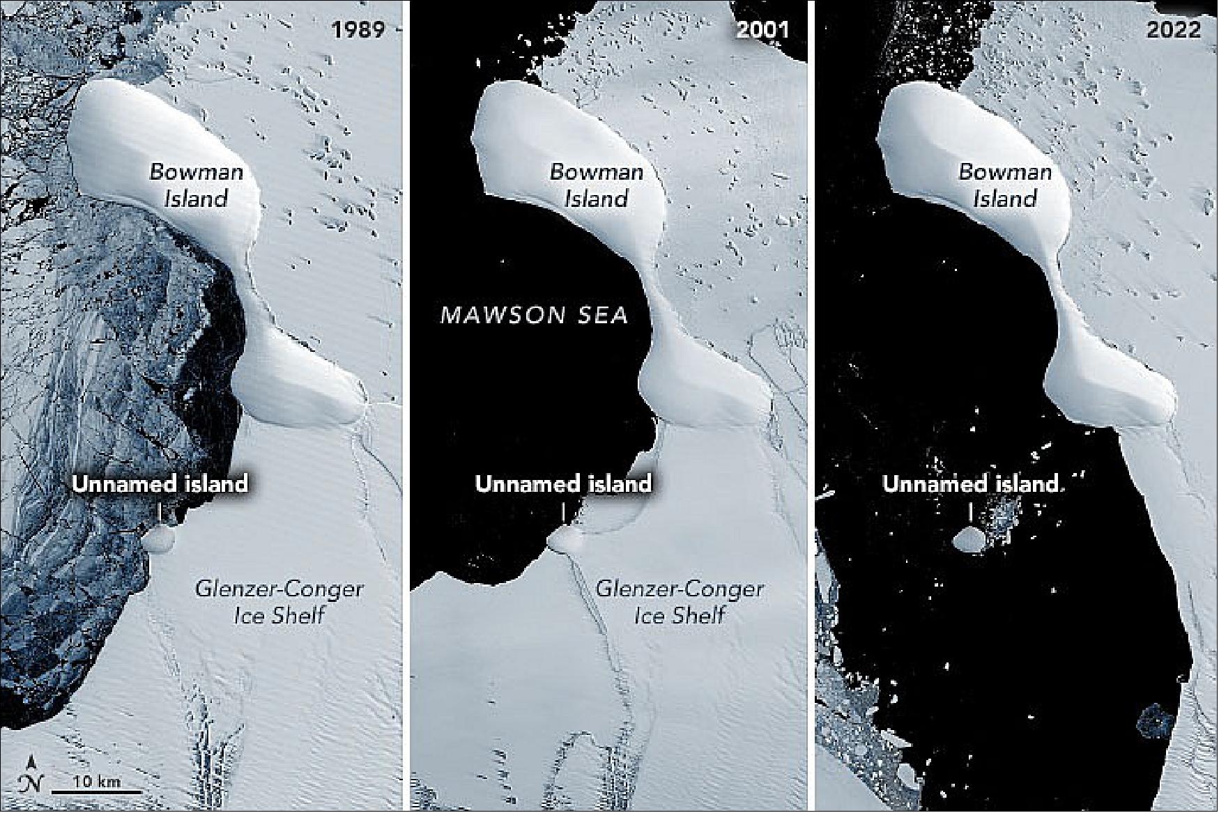
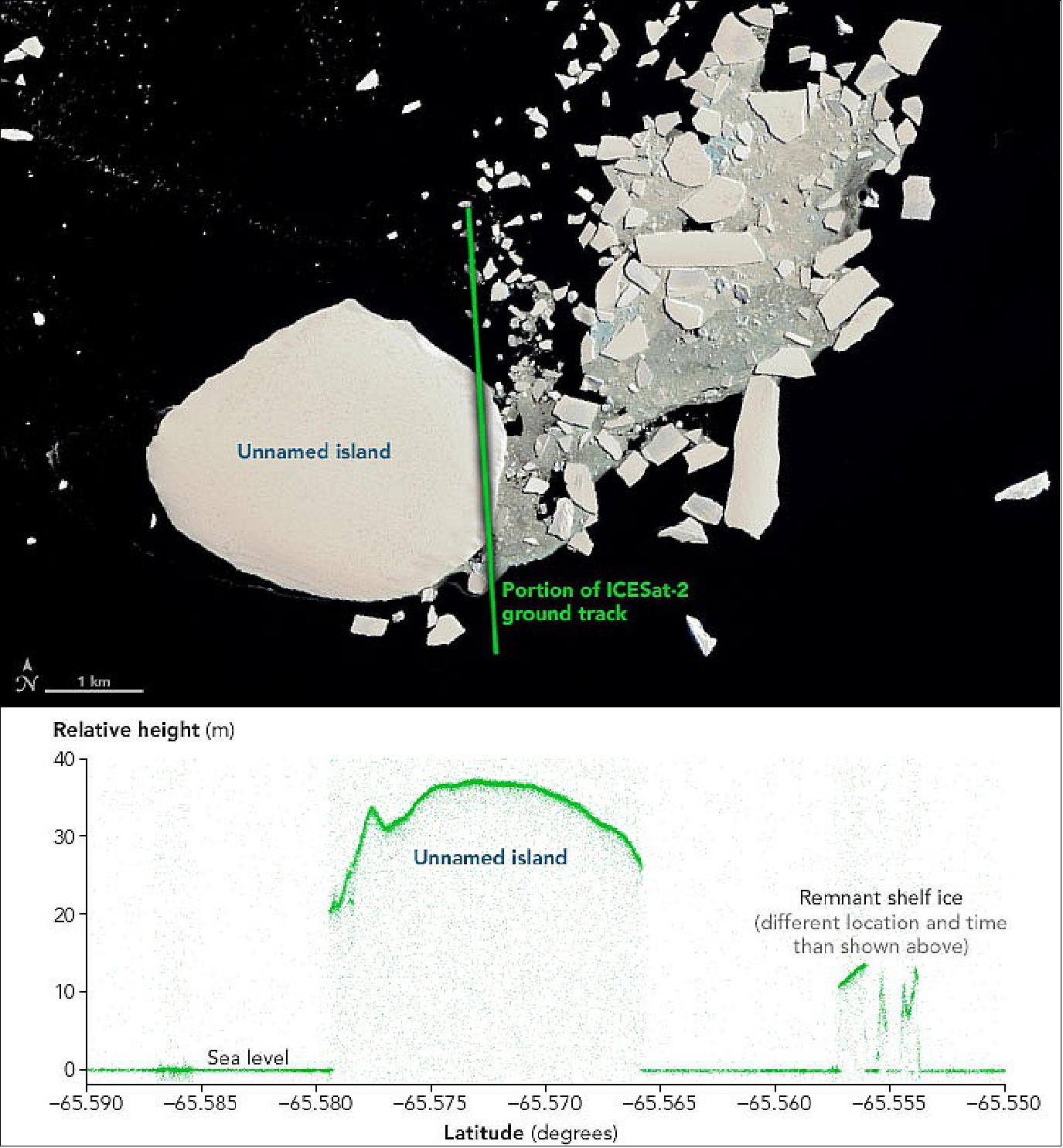
• April 27, 2022: The eastern Antarctic coast lost most of the Glenzer and Conger ice shelves, potentially revealing a new, unnamed island. If confirmed, the unnamed island would be one in a series of islands exposed in recent years as portions of the floating glacial ice hugging the continent’s coast have disintegrated. 48) Scientists are unsure if solid ground exists beneath the snow and ice, as it could be a "self-perpetuating" ice island, balancing snowfall and underwater melting. If disrupted, it could thin and drift away. In 2019, the U.S. Board on Geographic Names recognised Icebreaker Island, which in 1996 became isolated from the Larsen B Ice Shelf along the Antarctic Peninsula. And in 2020, researchers on a ship-based expedition discovered a small, rocky island capped with ice that may have been part of Pine Island Glacier’s ice shelf.
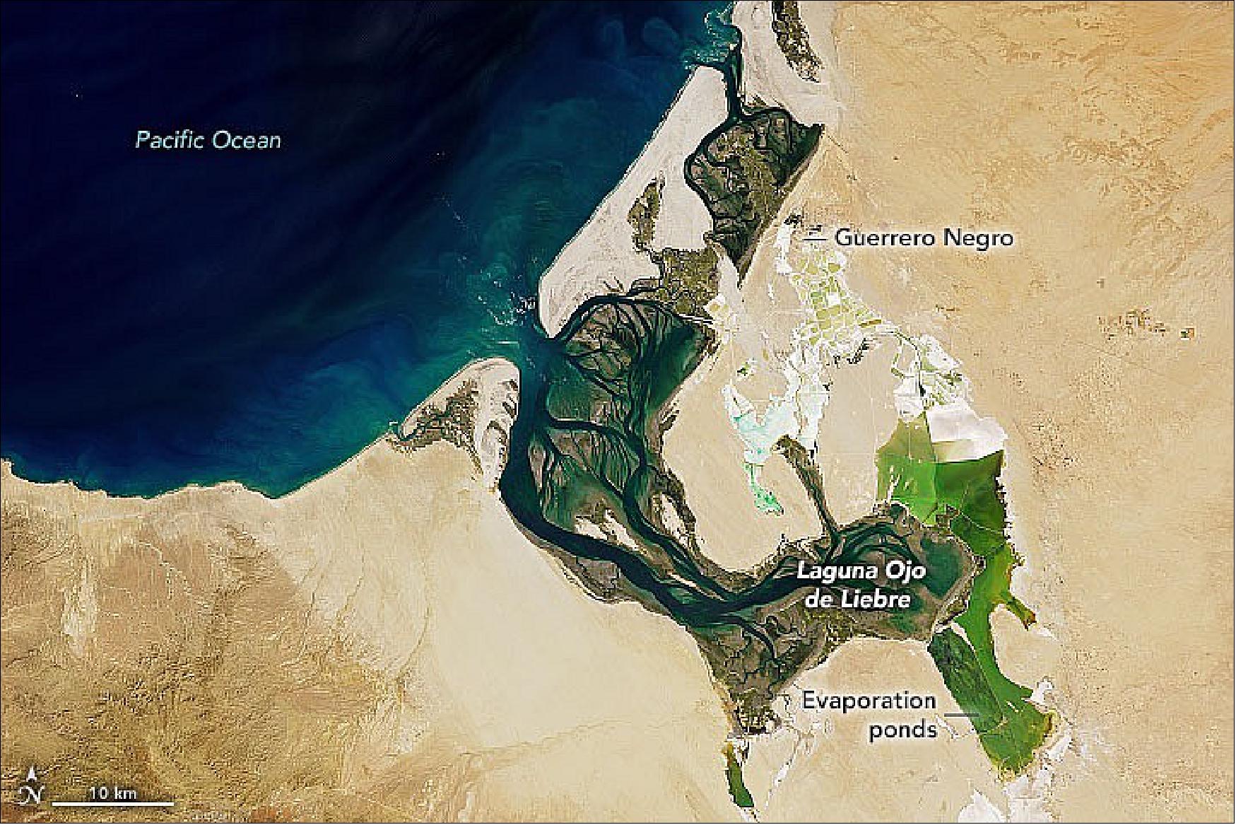
• April 25, 2022: Laguna Ojo de Liebre on the Pacific coast of Mexico is the site of one of the largest saltworks in the world. The lagoon and saltworks lie near the town of Guerrero Negro, about halfway between the U.S-Mexico border and the southern tip of the Baja California peninsula. 49) In addition to salt production, the area also supports commercial fisheries and ecotourism. The lagoon is part of the Vizcaíno Biosphere Reserve. This UNESCO World Heritage Site, the largest protected area in Mexico, is an important whale sanctuary for the North Pacific grey whale. The whales migrate between their winter nursery grounds in the lagoons and their summer feeding grounds in the Chukchi, Beaufort, and Bering seas. The lagoons also host countless other marine species and migrating birds.
• April 21, 2022: According to data from the National Phenology Network, the first leaves and flower blooms in eastern Tennessee came in late-March and early April, about a week earlier than usual. Seasonal greening comes earlier to low-lying parts of the Tennessee Valley, as grasses, bulbs, herbaceous perennials, and shrubs awake from their winter slumber. Elevation effects keep the tops of the region’s long ridges cool and brown in early spring. On average, every 1,000 feet (300 meters) of increased elevation amounts to a 3º Fahrenheit (5º Celsius) decrease in temperature. Across the state of Tennessee, average annual temperatures vary from over 62°F (16°C) in the extreme southwestern part of the state to 46°F (8°C) atop the highest peaks in the east. Clinch Mountain, for instance, rises 1,018 feet (310 meters) above the surrounding landscape at a lookout tower in Hawkins County.
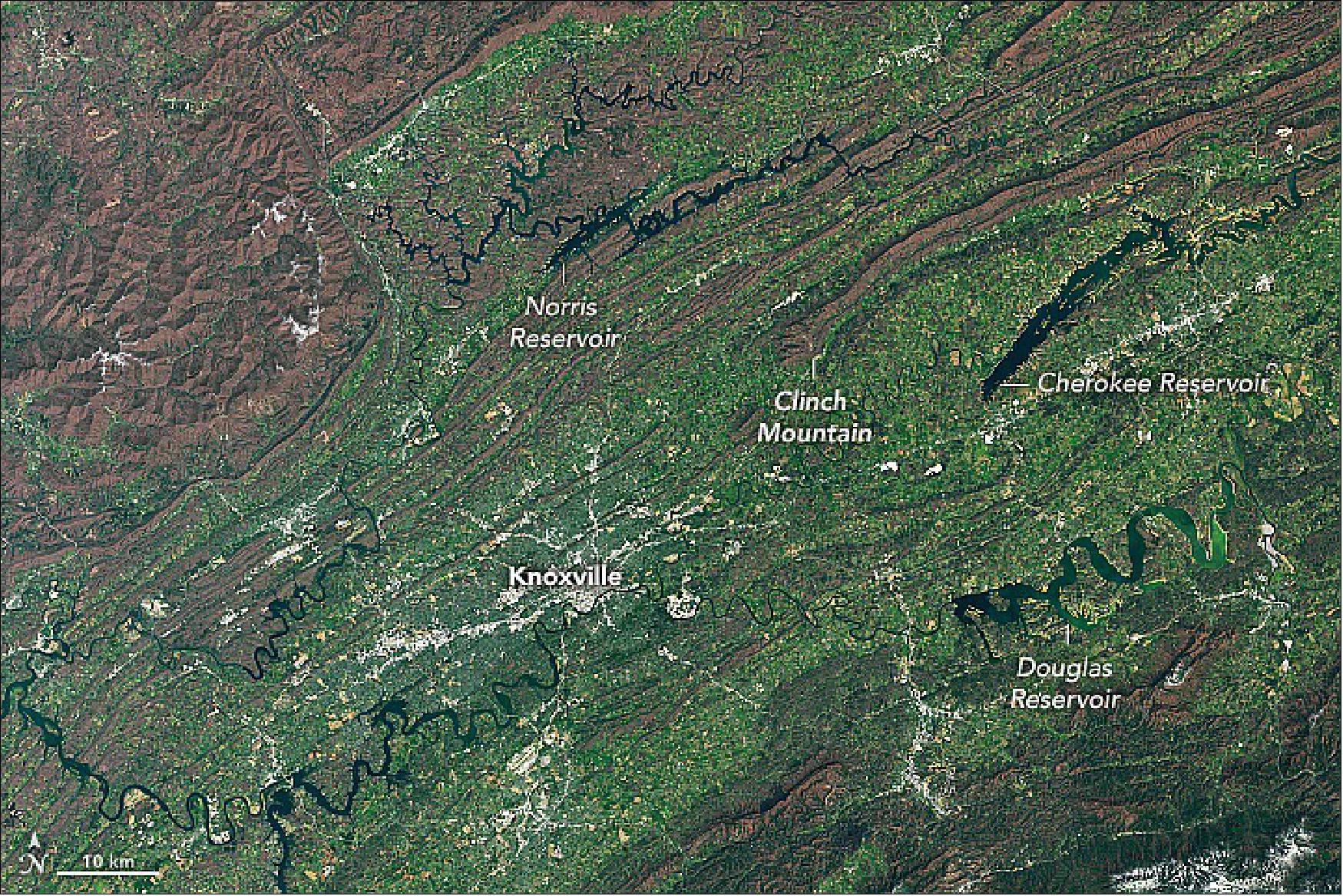
- The image also highlights some of the hydropower resources found in the Tennessee Valley, including Norris, Cherokee, and Douglas reservoirs. Begun in October 1933 and finished in March 1936, Norris Dam was the first hydroelectric project completed by the Tennessee Valley Authority (TVA). The public power company was created in 1933 in response to the Great Depression and headquartered in Knoxville. Tennessee is the third-largest hydroelectric power producing state east of the Rocky Mountains (after New York and Alabama) according to U.S. Energy Administration Statistics. Tennessee is home to 26 hydroelectric power plants, plus a large pumped storage hydroelectric facility. Hydroelectric power provides 13 percent of the state’s total electricity generation and almost 90 percent of the stat’s renewable generation.
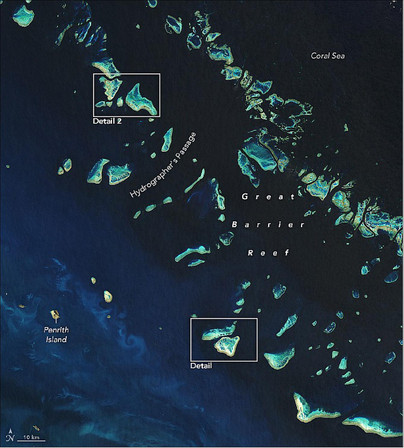
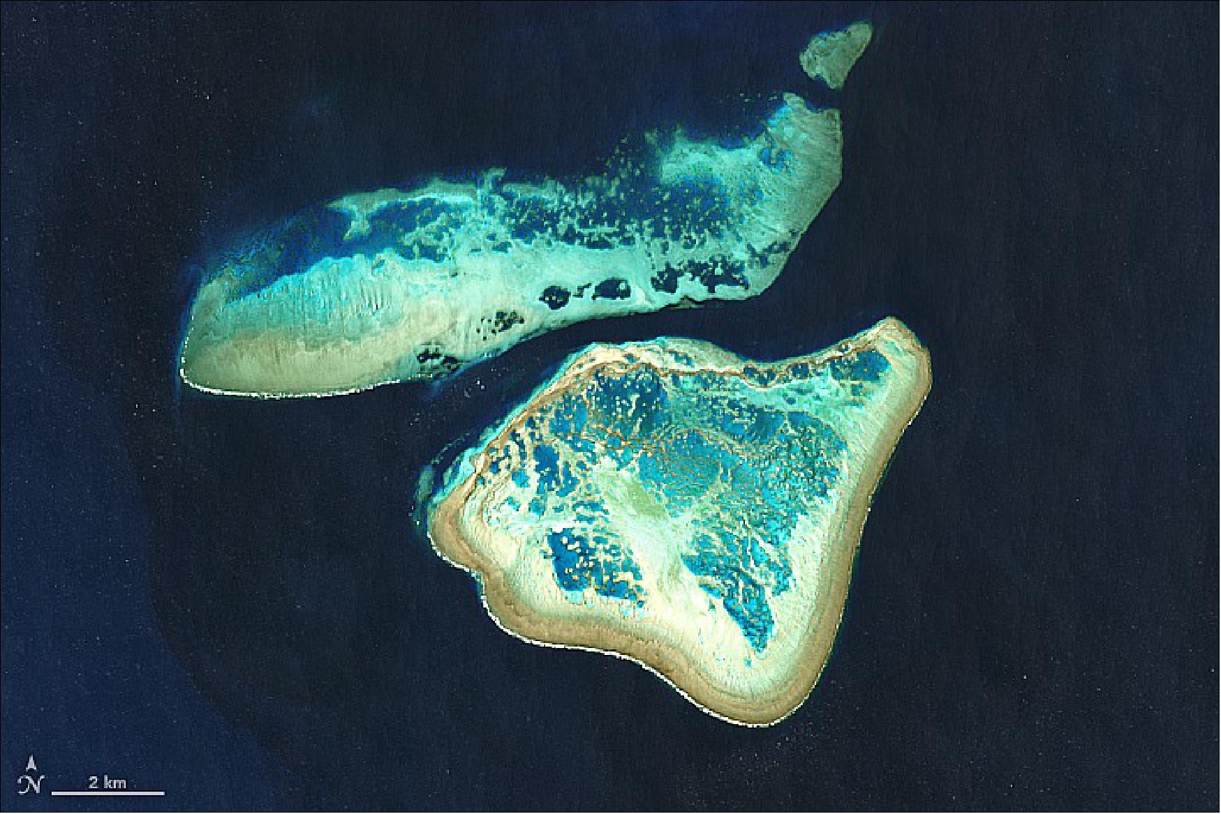
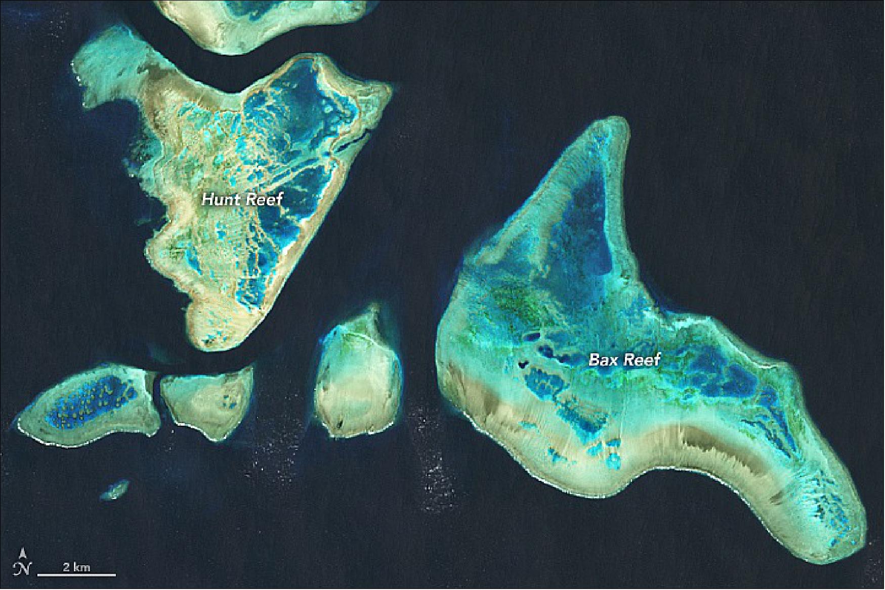
• April 16, 2022: Global sea level rise will also bring changes to the Great Barrier Reef system, as research shows it has in the past. The Great Barrier Reef has declined, migrated, and rebounded many times before. 51) The University of Sydney-led research team drilled cores in the reef at Hydrographer’s Passage off Mackay and at Noggin Pass off Cairns. They found multiple landward and seaward migrations caused by sea level change, which is the primary driver of reef growth and migration. Some fossil reef structures and the shelf upon which the modern reefs have been built are several hundred thousand years old. However, the living reef that we see today is less than 10,000 years old. It is just the latest of at least five reefs that have grown here over the past 30,000 years, according to research reported in 2018. 52)
- During ice ages, massive amounts of water are locked up in glaciers and ice sheets; sea level drops and sea surface temperatures cool. During interglacial periods, sea levels rise and water temperatures warm. As sea level changes, coral polyps will build up their calcium carbonate skeletons to stay within the photic zone, the upper ocean layers where sunlight can penetrate. At times, the reef tracked rising sea level, growing vertically up to 20 meters (65 feet) per thousand years and migrating laterally at 1.5 meters (5 feet) per year, the researchers found. At other times, however, sea level rose too quickly for the corals to keep up and the reefs were drowned. Rapid sea level drops also caused some die-offs by exposing the reef above the water surface.
• April 14, 2022: In March 2011, an earthquake and tsunami damaged nuclear reactors and released radioactive material from the Fukushima Daiichi Nuclear Power Plant in northeastern Japan. More than a decade later, the area around the damaged power plant has become a hub of renewable energy production. 53) Many fields no longer suitable for farming now gleam with rows of solar panels due to a multibillion-yen investment in renewable energy. Government and industry financiers started pursuing plans to develop 11 solar farms and 10 wind farms on abandoned or contaminated land around Fukushima, according to news reports.
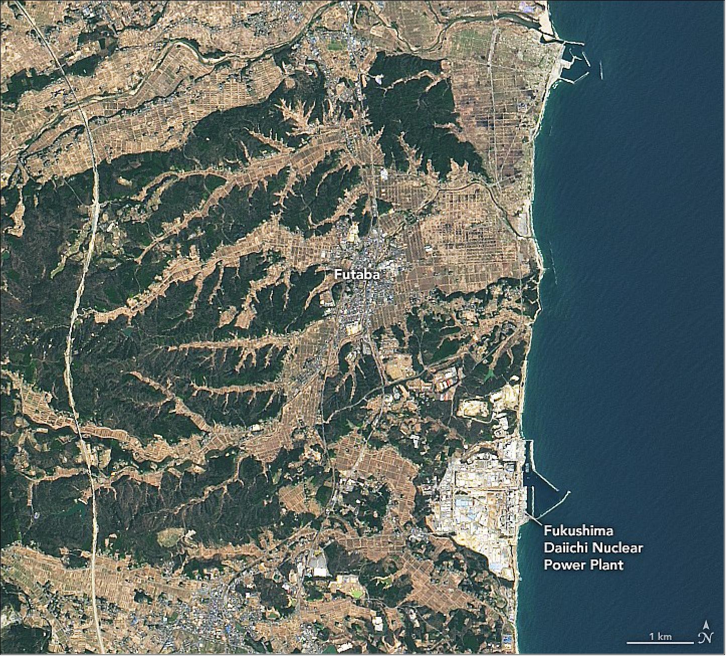
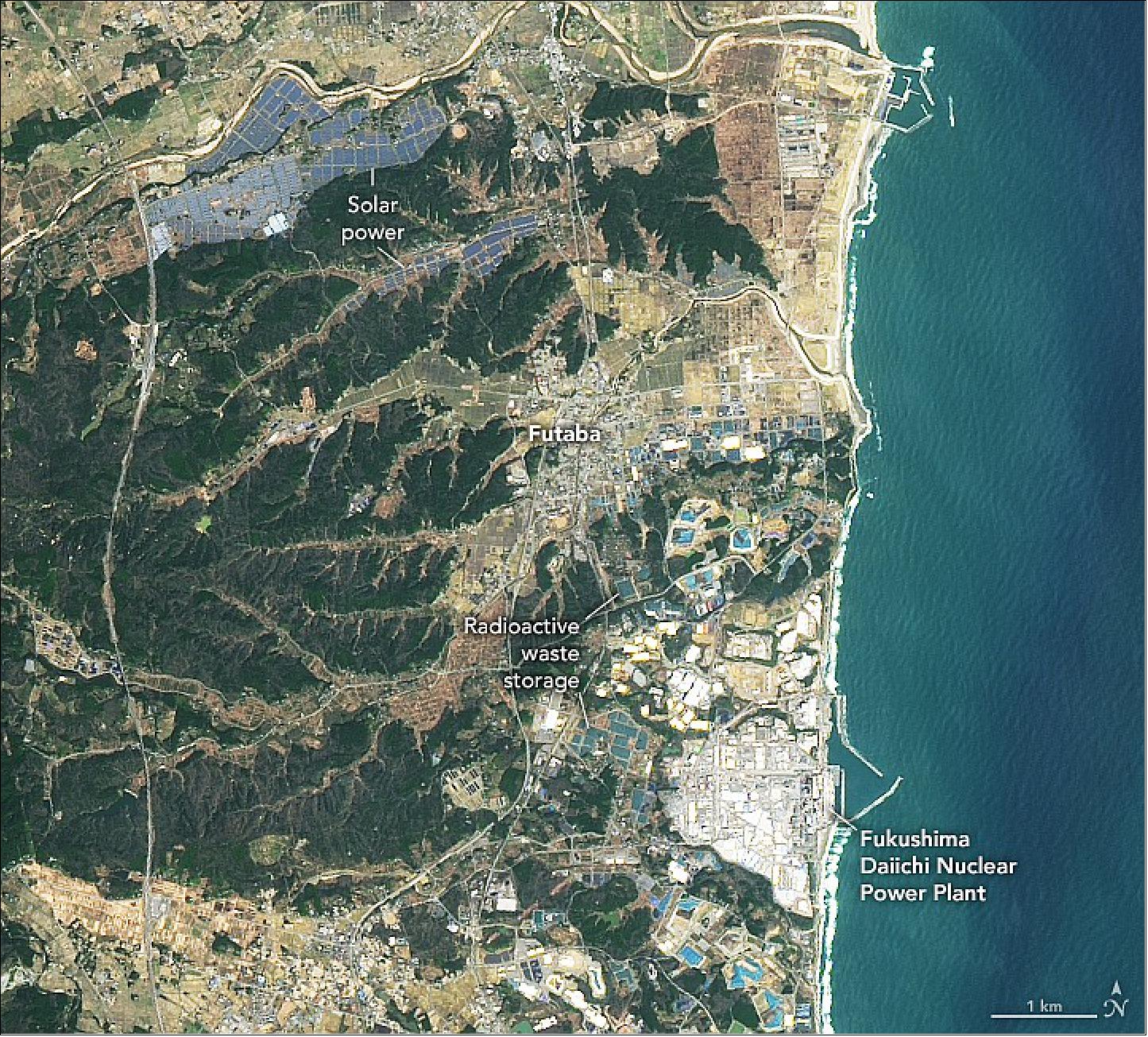
- In 2014, Fukushima prefecture announced a goal of having all of its energy come from renewable sources by 2040. Local leaders have made considerable strides, with 43 percent of energy coming from renewable sources by 2020, up from 24 percent in 2011. Prior to the accident at Fukushima, nuclear power provided about one quarter of Japan’s electricity. This share plummeted to less than 1 percent after the accident. The rapid expansion of renewable energy production has helped compensate for the change, but the share of natural gas and coal has increased significantly as well, according to data from the U.S. Energy Information Administration. In recent years, the use of nuclear power in Japan has also rebounded, accounting for 7 percent of electricity generation in 2019.
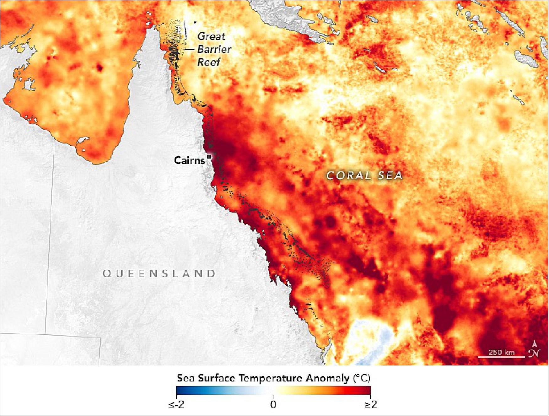
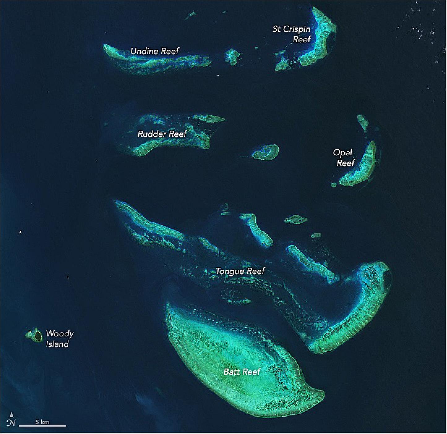
• April 7, 2022: After conducting aerial surveys of more than 750 reefs in the marine park, the Australian government’s Great Barrier Reef Marine Park Authority confirmed in late March that a mass bleaching event had occurred. It was the sixth such widespread bleaching event of the reef since 1998. 54) La Niña is the cooler phase of the El Niño Southern Oscillation, during which coupled atmospheric and ocean circulation patterns in the tropical Pacific alter global climate. conditions typically bring more rain and cooler temperatures over the reef, according to Australia’s Bureau of Meteorology. The Great Barrier Reef, spans 346,000 km² off Queensland, Australia. Mass coral bleaching events, caused by sustained warm sea surface temperatures (SSTs), occur when heat stress forces corals to expel symbiotic zooxanthellae, leaving them "bleached." Major bleaching occurred in 1998, 2002, 2016, 2017, 2020, and again in 2021 during a La Niña year, despite slightly cooler global temperatures. Bleaching impacted all reef areas, most severely in the north and center, correlating with satellite heat data. Climate warming is intensifying and prolonging bleaching events globally, including the 2014–2017 event, the longest and most damaging recorded. Designated a UNESCO World Heritage site in 1981, the reef remains one of Earth's richest ecosystems but faces mounting threats.
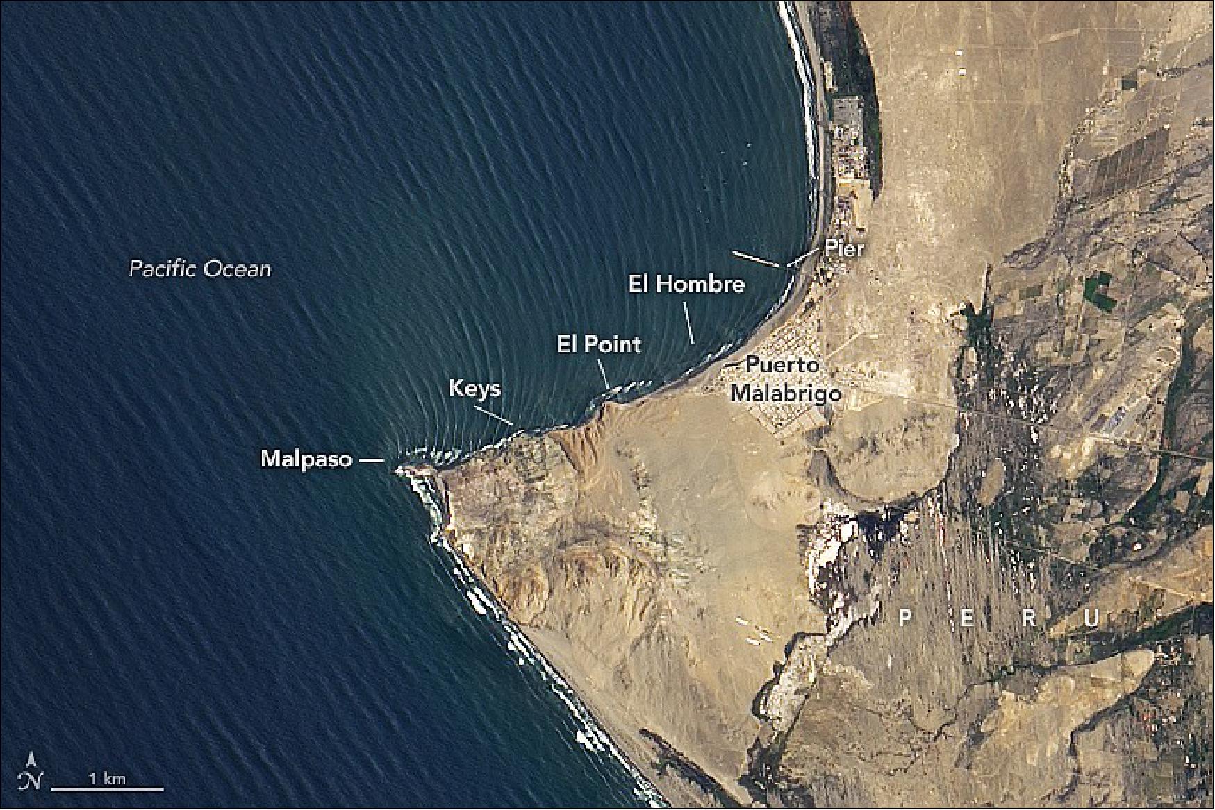
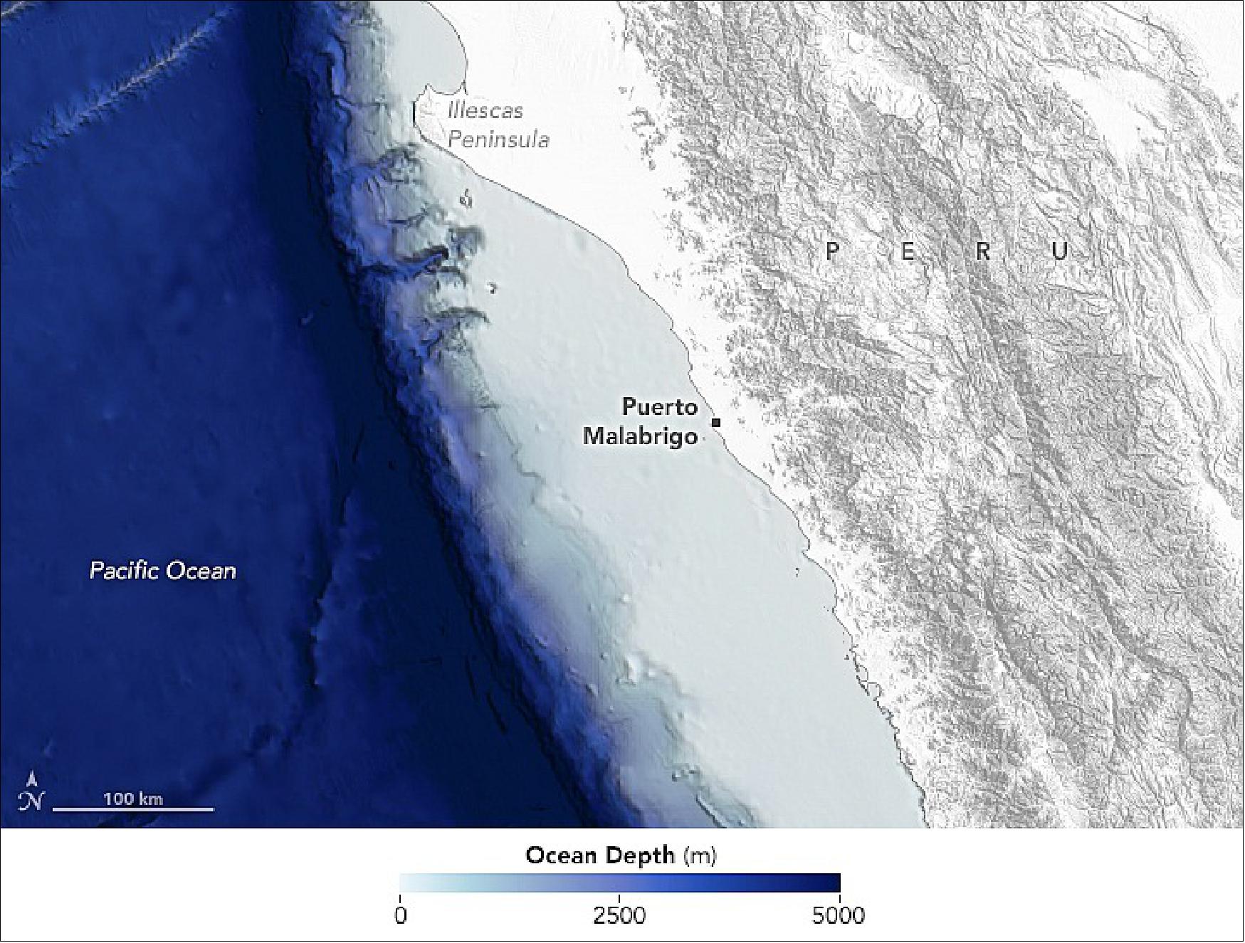
• April 1, 2022: The waters off the Pacific coast of northern Peru routinely build what has been called the world’s longest wave. There’s no way to know for sure, but the seemingly endless waves that roll up to the fishing town of Puerto Malabrigo (Chicama) are legendary among surfers. While some famous wave breaks around the world can be ridden for seconds, the breaks at Chicama can be ridden for minutes. 55) The breaks that surfers most frequently ride begin along the cape that juts out into the Pacific. This is where four points, Malpaso, Keys, El Point, and El Hombre, trigger the crest of a swell to overturn and peel as it approaches the shallowing shore. Chicama’s waves break left, which means they peel from left to right from the perspective of an observer on the shore. Large swell is most consistent from March through November, during which time some of the sections occasionally connect.
• March 13, 2022: A University of Kentucky horticulture professor developed the first plastic greenhouse in the 1950s. Plastic greenhouses are an effective and inexpensive way to increase farm yields by extending the growing season and exerting control over temperature and lighting conditions. 56) The use of plastic on farms has become so common in recent decades that there is a term for it, plasticulture. While there’s still no easy, globally consistent way of tracking how far plasticulture has spread, there are plenty of signs that its footprint is significant. By some estimates, plastic greenhouses now cover as much as 3 percent of China’s farmland. South Korea, Spain, and Turkey also use significant amounts of agricultural plastic for greenhouses.
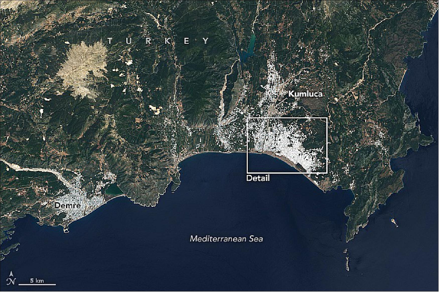
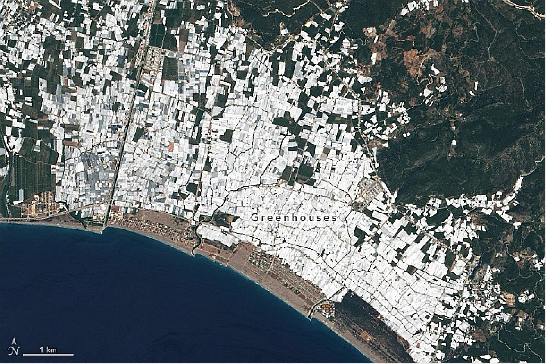
- Tomatoes, peppers, and cucumbers are commonly grown in greenhouses in this area. With 772 km2 (298 square miles) of land covered by greenhouses, Turkey ranks fourth in the world in greenhouse cultivation, according to one team of researchers from Çukurova University. That is an area roughly the size of New York City.Farmers use thin sheets of plastic mulch to protect plants from pests and weeds, with China leading in usage, covering 13 percent of its farmland. However, plastic pollution poses environmental risks, producing toxins when burned and microplastics in soil and water. Global agricultural plastic demand is projected to rise from 6.1 million tons in 2018 to 9.5 million tons by 2030.
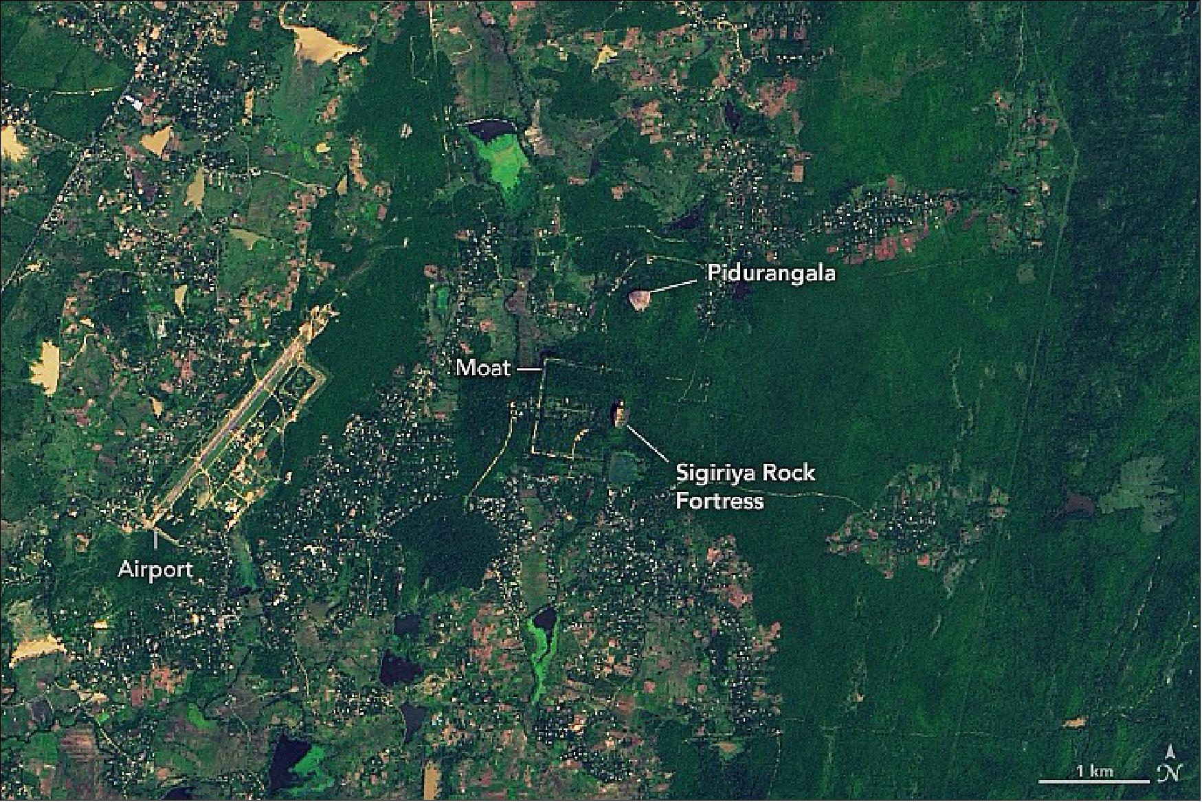
• March 5, 2022: Two billion years ago, the piece of land that now makes up north central Sri Lanka had several active volcanoes. Though most of these ancient features have been worn away, their remnants persist in the form of towering pillars of rock that soar above the surrounding plain. 57) In the fifth century, King Kasyapa built a palace and fortress atop Sigiriya, featuring a moat and water garden. Now a UNESCO World Heritage Site, it attracts up to one million visitors annually. Nearby Pidurangala, where displaced Buddhist monks relocated, houses a temple complex with ancient sculptures and paintings. Both Sigiriya and Pidurangala are volcanic plugs, formed from hardened magma resistant to erosion, once connecting magma chambers to surface vents.
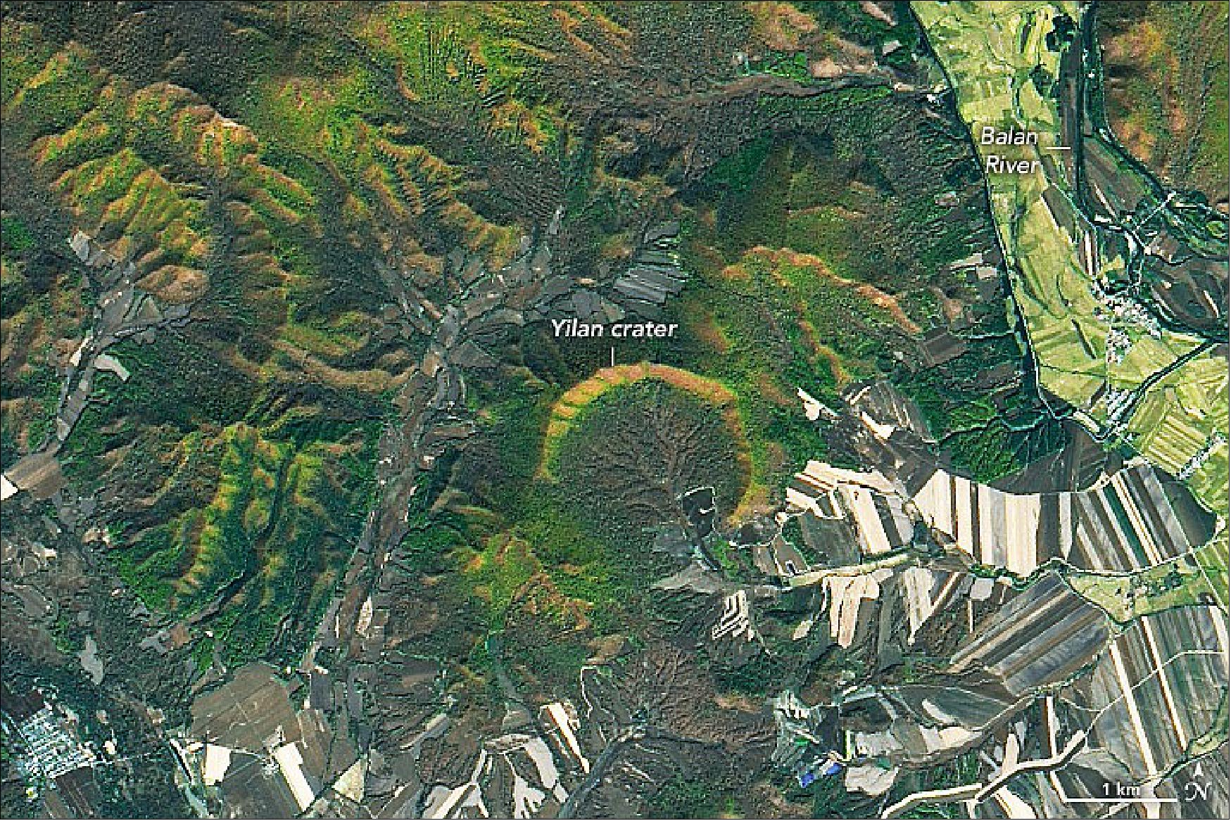
• February 27, 2022: Despite China’s large land area, only one impact crater, the relatively small Xiuyan crater in Liaoning province, had been discovered there prior to 2020. In 2021, a team of geologists found another crater northwest of Yilan in Heilongjiang Province. The crater was discovered in the heavily forested Lesser Xing’an mountain range, where local residents knew it as “Quanshan,” or “circular mountain ridge.” 58) The Yilan crater, 1.85 km wide, is Earth’s largest crater under 100,000 years old, formed 46,000–53,000 years ago. It exceeds Arizona’s Meteor (or Barringer) Crater in size. The impact struck 200-million-year-old Jurassic granite, leaving lake sediments, shattered granite, shocked quartz, and impact glass. Drilling revealed evidence confirming its impact origin. While the southern rim is missing, lakebed sediments suggest it remained intact long enough to accumulate rich organic soil, now supporting farms, swamps, and wetlands.
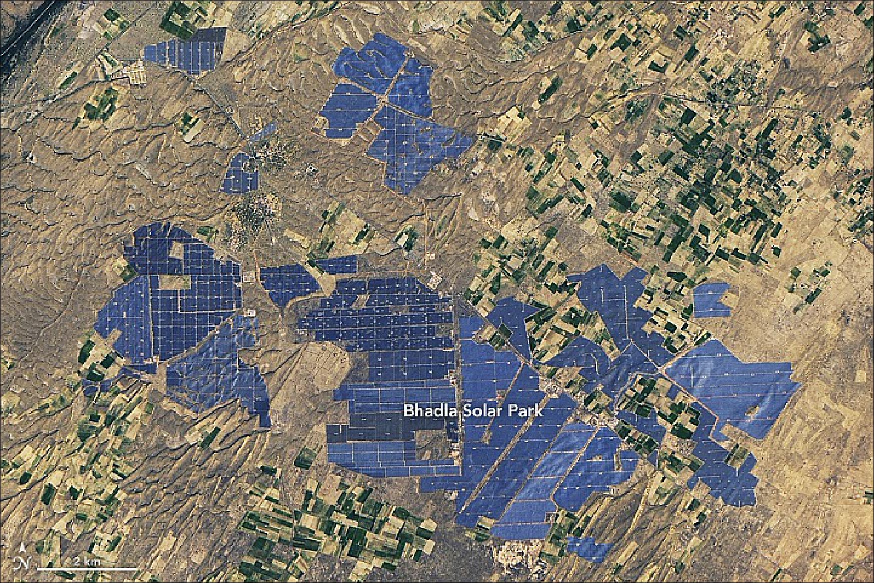
• February 19, 2022: The abundance of open space and sunshine make Phalodi township in India’s Thar desert, western Rajasthan, an ideal place for harvesting solar power. 59) Bhadla Solar Park spreads across more than 5700 hectares (57 km2 or 22 square miles), an area about one-third the size of Washington, D.C. It has a total capacity of 2245 megawatts, among the largest solar parks in the world. Its presence recently helped Rajasthan overtake Karnataka as the Indian state with the largest installed solar capacity, according to Mercomm India.Though the area’s consistently clear skies mean sunlight is abundant, frequent dust storms pose an engineering challenge because they coat the panels with layers of minerals and sand that hamper electricity production. Some operators have chosen to unleash thousands of cleaning robots on the panels, a tactic designed to cut manual labor needs and reduce the amount of water required for cleaning. Some recent research suggests that Landsat imagery could assist such systems by helping companies identify dust buildup and optimise cleaning operations.
• February 16, 2022: A severe drought that began in November 2021 has worsened significantly, prompting officials in Portugal to limit the use of five hydroelectric dams for power production and irrigation after some reservoirs reached significant lows. 60) In Spain, the driest January in 20 years has depleted reservoirs to below 45 percent of their capacity, with Andalusia in the south and Catalonia in the northeast experiencing the worst drought conditions, according to Spain’s State Meteorological Agency. The dry spell in Portugal started in November 2021 and worsened in December; by late January, nearly all of the country was experiencing moderate to severe drought conditions, according to the Portuguese Institute of Meteorology. In the middle of what would normally be the wet winter season, 54 percent of the country was experiencing moderate drought, 34 percent was in severe drought, and 11 percent was in extreme drought.
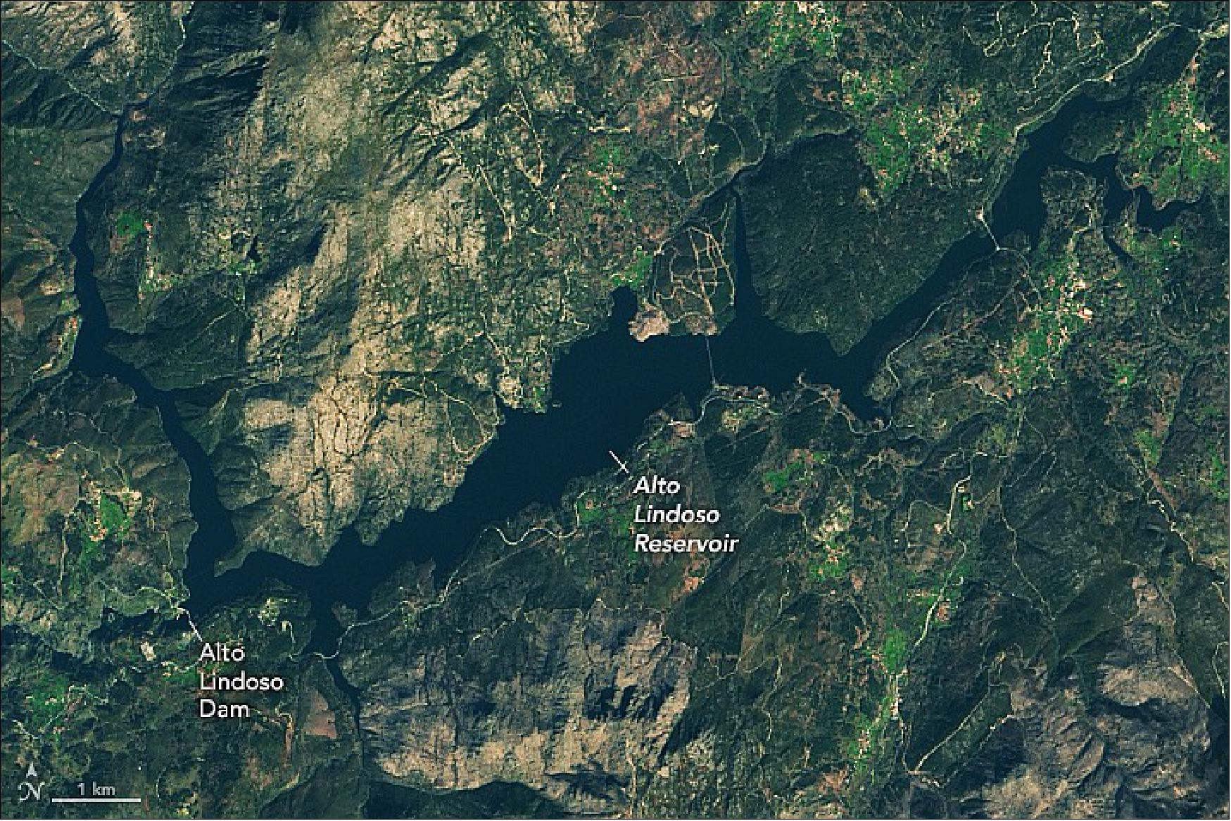
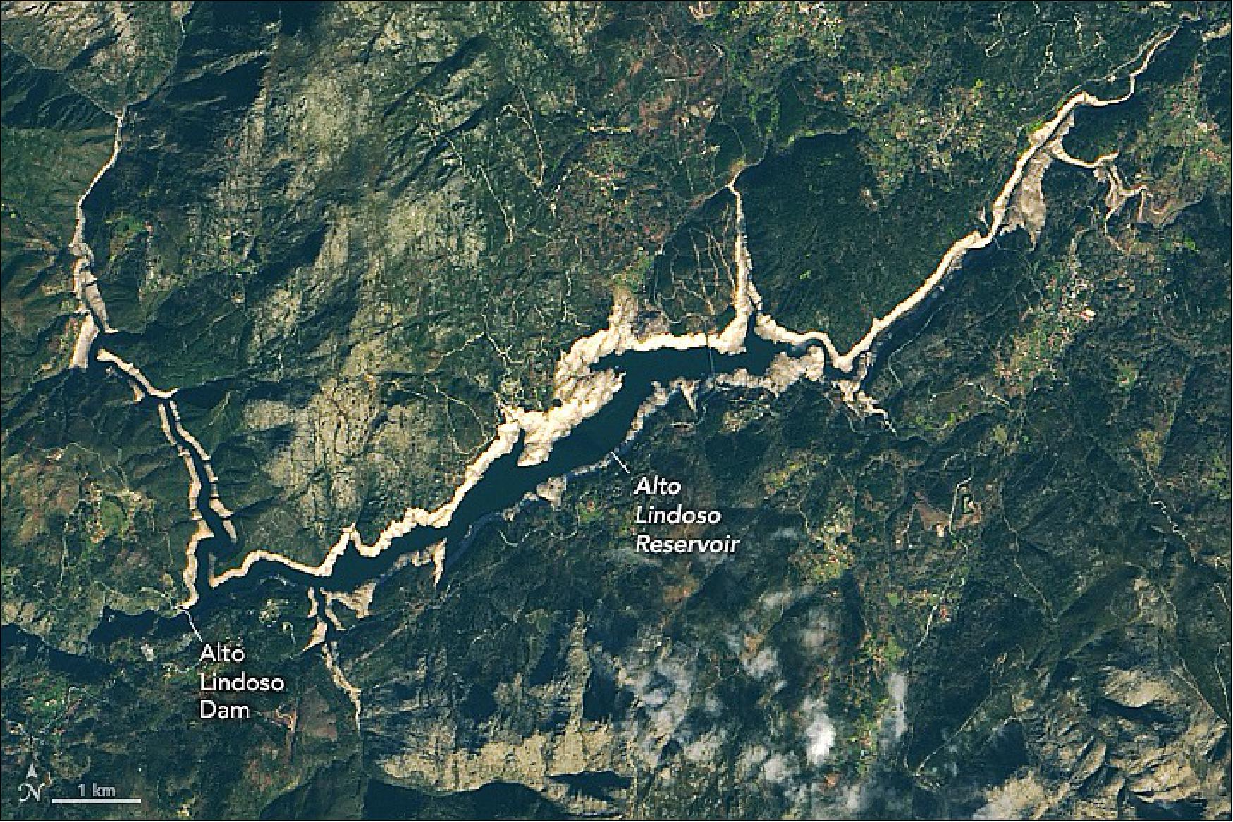
- In early February, Portuguese officials announced the Alto Lindoso and three other dam-reservoir systems (not including Alto Rabagão) will limit water usage for power generation to a few hours a week. Portugal has a significant hydropower program with about 60 dams around the country generating 10.6 Terawatt-hours of power in 2019, about 30 of the country's energy and half of its renewable energy. One other dam, Bravura, will not be used for irrigation. Across the region, the lack of precipitation has left many farmers struggling to find sufficient grazing land for their livestock. The drought is also visible in satellite gravimetry observations made by the Gravity Recovery and Climate Experiment Follow-On (GRACE-FO) satellites, which measure groundwater storage and soil moisture.
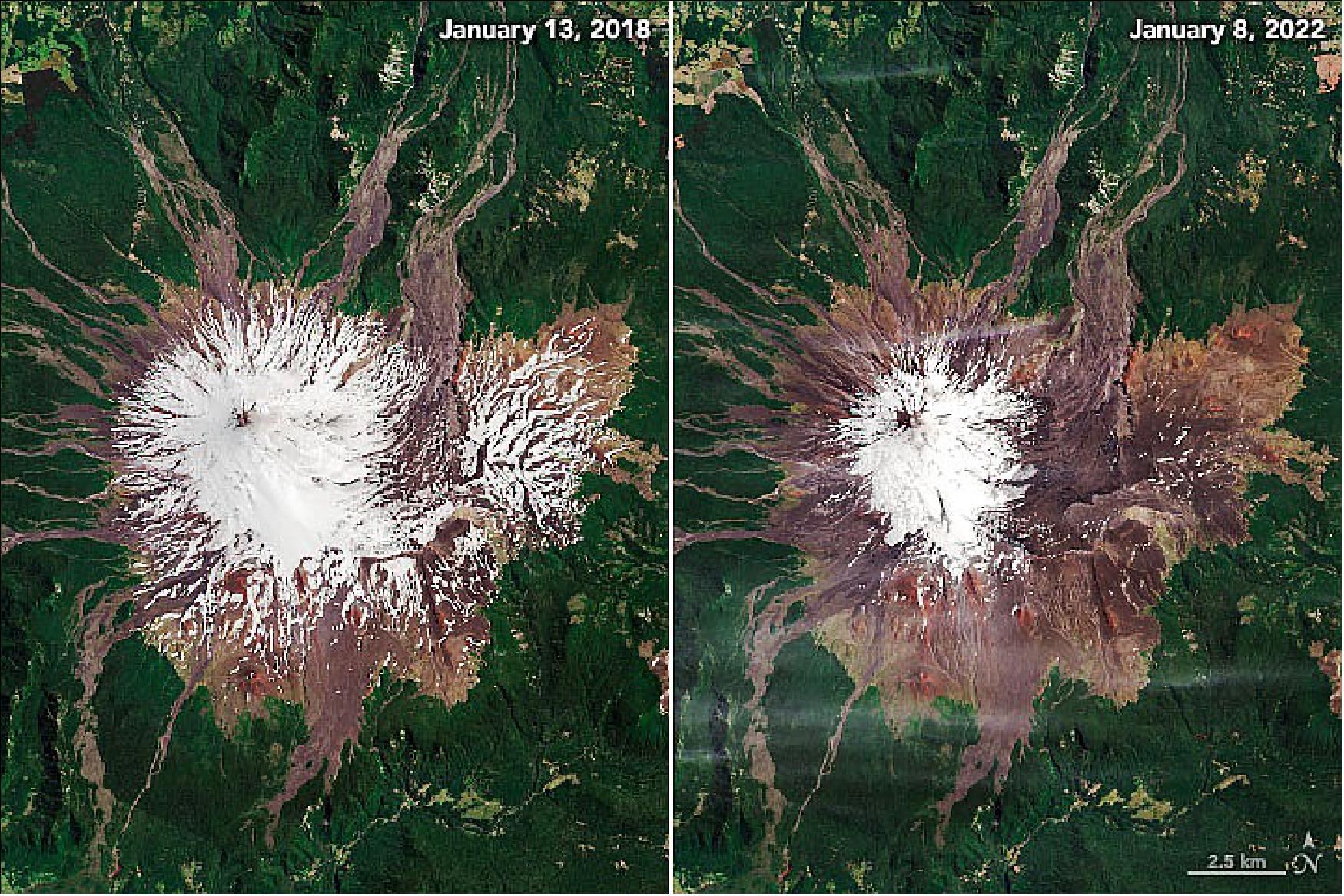
• February 15, 2022: Pucón, Chile, is located between a glacier-carved lake and snow-capped volcano. Visible from nearly anywhere in the town, the stark-white slopes of Villarrica volcano form a majestic backdrop. But in summer 2022, the backdrop lacked its typical luster as the volcano’s slopes appeared more bare than usual. 61) Villarrica is part of a chain of volcanoes that characterise the southern Andes Mountains in Chile’s Araucanía and Los Ríos regions. Areas to the north, in central Chile (including Santiago, 675 km) are quite a bit drier; areas to the south, in the Patagonia region, are more humid. The area around the volcanoes usually receives from 100 to 200 cm (39 to 79 inches) of precipitation per year, most of which falls in winter. But 2021 was exceptionally dry. Other volcanos in the area are also low on snow this summer, including Mocho-Choshuenco located 55 km (34 miles) south-southwest of Villarrica. Scientists used Landsat images to study snow cover trends on this volcano and found that snow that once persisted year-round at middle elevations is now seasonal. The dry weather in 2021 is part of a continuing megadrought that has persisted in central Chile for more than a decade.
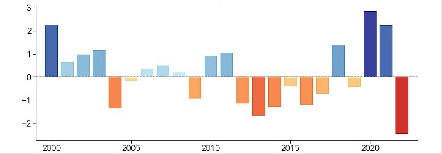
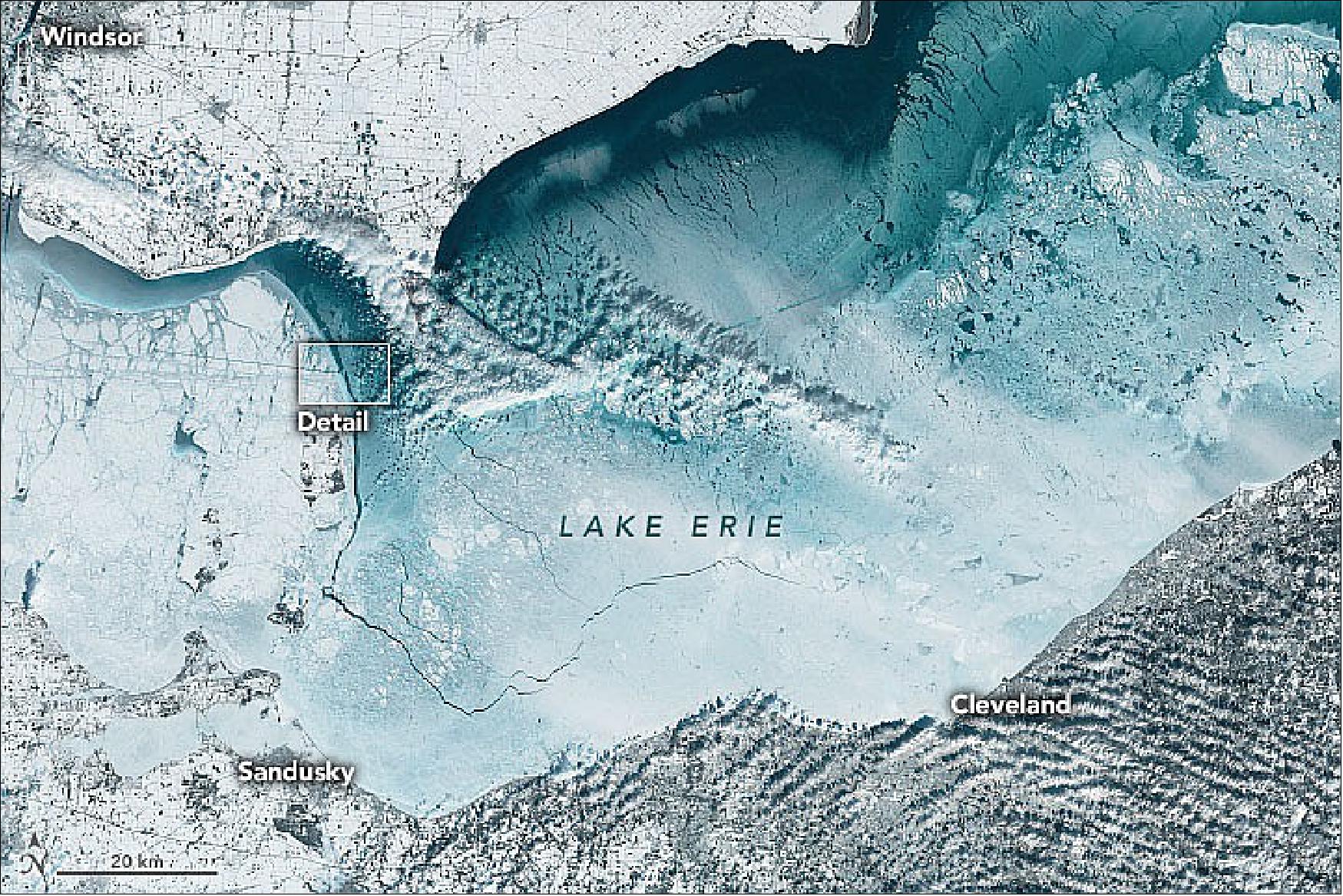
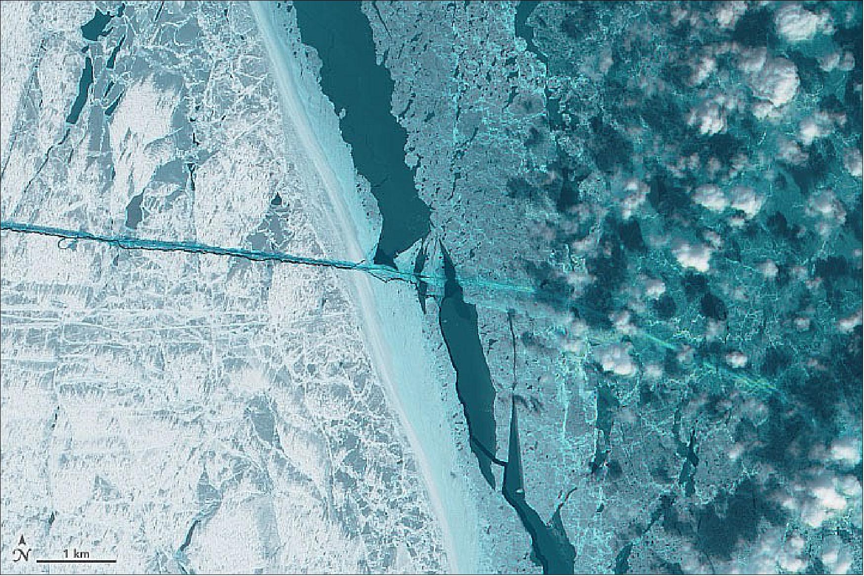
• February 9, 2022: In late January 2022, Lake Erie nearly froze over entirely, with ice cover growing well beyond the seasonal average to reach 94 percent. By February 3, the ice cover had dropped to about 62 percent before rising again to 90 percent by February 5. 62) The extent and thickness of ice on the Great Lakes are mainly influenced by air temperature and wind. As the shallowest of the Great Lakes, Erie has the highest annual maximum ice cover, regularly reaching more than 80 percent. Three times in the past half century Lake Erie reached 100 percent ice cover: 1978, 1979, and 1996.
- Conditions on the lake are not only highly variable from year to year, but also day to day. The first week of February 2022 brought a heavy snowstorm, wildly varying wind speeds and directions, and days of continuous cooling. As a result, the ice extent across the Great Lakes rapidly expanded. On February 1, the average ice cover across all the lakes was 12 percent; two days later it had expanded to 28 percent; and by February 6 it was 43 percent. (Between 1973–2021, the Great Lakes’ annual average maximum ice coverage was 53.1 percent.)
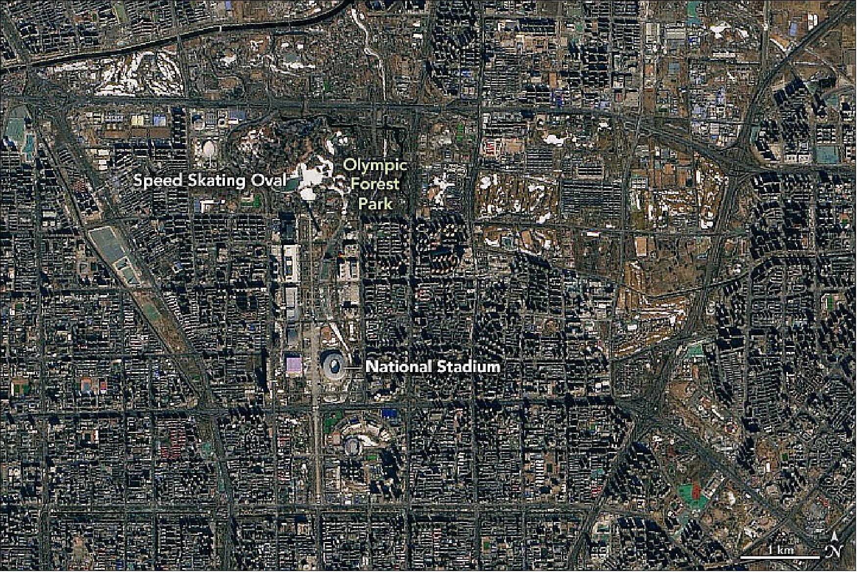
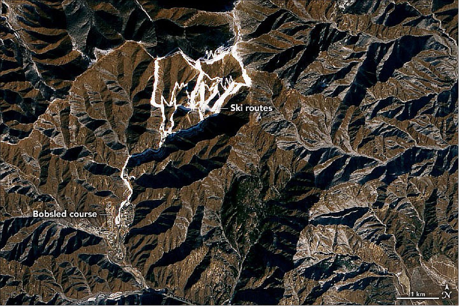
• February 7, 2022: Beijing, surrounded by mountains, hosted the 2022 Winter Olympics, using the terrain for alpine skiing, snowboarding, and sliding events 63) Artificial snow, made with water from Foyukou and Baihepu reservoirs, covered steep slopes with inclines up to 68 degrees. Satellite imagery from January 29, 2021, shows snow-covered trails amid brown hills near the Yanging Olympic Village. The artificial snow was easy to spot in satellite imagery of the area. On January 29, 2021, the Operational Land Imager (OLI) on Landsat-8 captured an image of the downhill trails covered with artificial snow. The water used to make the snow gets piped in from the nearby Foyukou and Baihepu reservoirs. The alpine skiing routes, situated amidst mostly brown hillsides, have maximum inclines of 68 degrees, making this one of the steepest skiing venues in the world. Tracks from the sliding center are visible just to the southeast near the Yanging Olympic Village.
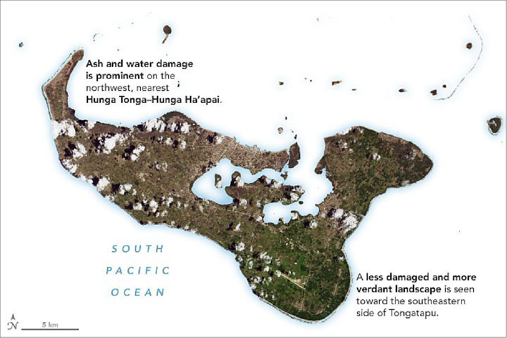
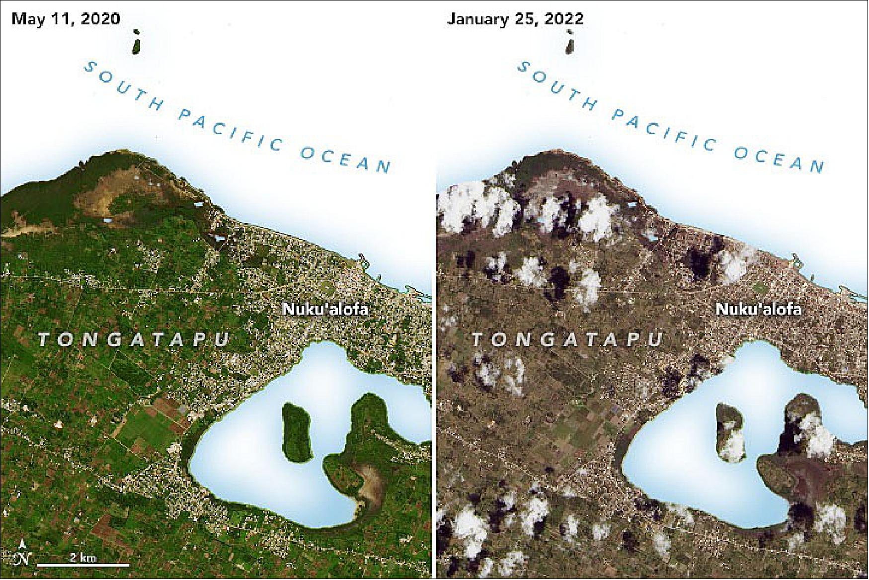
• January 31, 2022: Ever since the uninhabited volcanic island Hunga Tonga-Hunga Ha‘apai exploded in mid-January 2022, the people of Tonga have faced a gauntlet of hazards. 64) After the eruption, volcanic ash. blanketed Tonga's islands, turning lush green landscapes tan and gray. Satellite images from January 25, 2022, show ash covering much of Tongatapu, Tonga’s most populous island. Rare volcanic tsunamis followed, with waves up to 15 meters (49 feet) high, devastating several islands. The waves destroyed buildings, cars, and trees, damaged power lines, and killed three people, leaving hundreds of structures damaged or destroyed. (The full scene is available for download.)
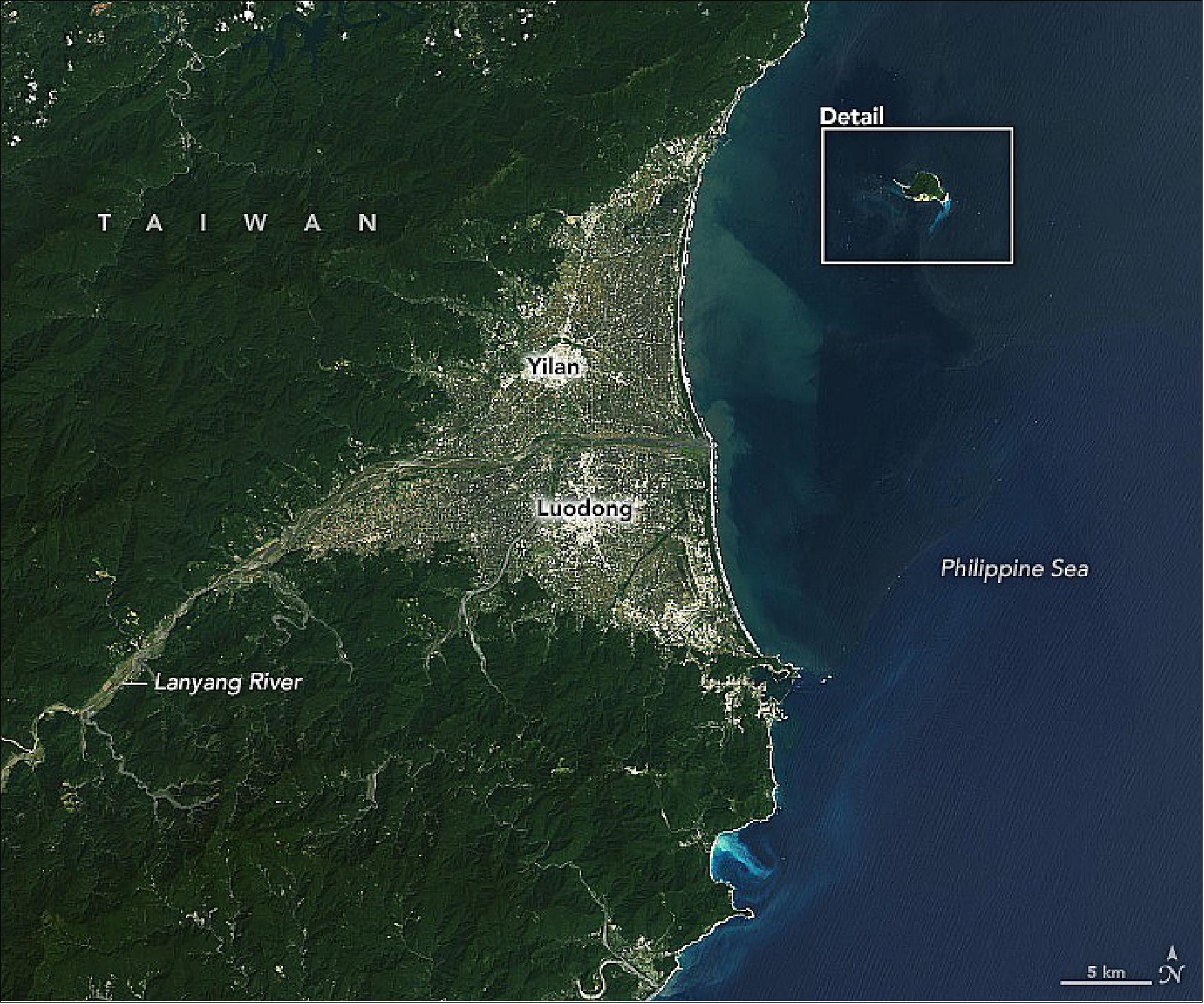
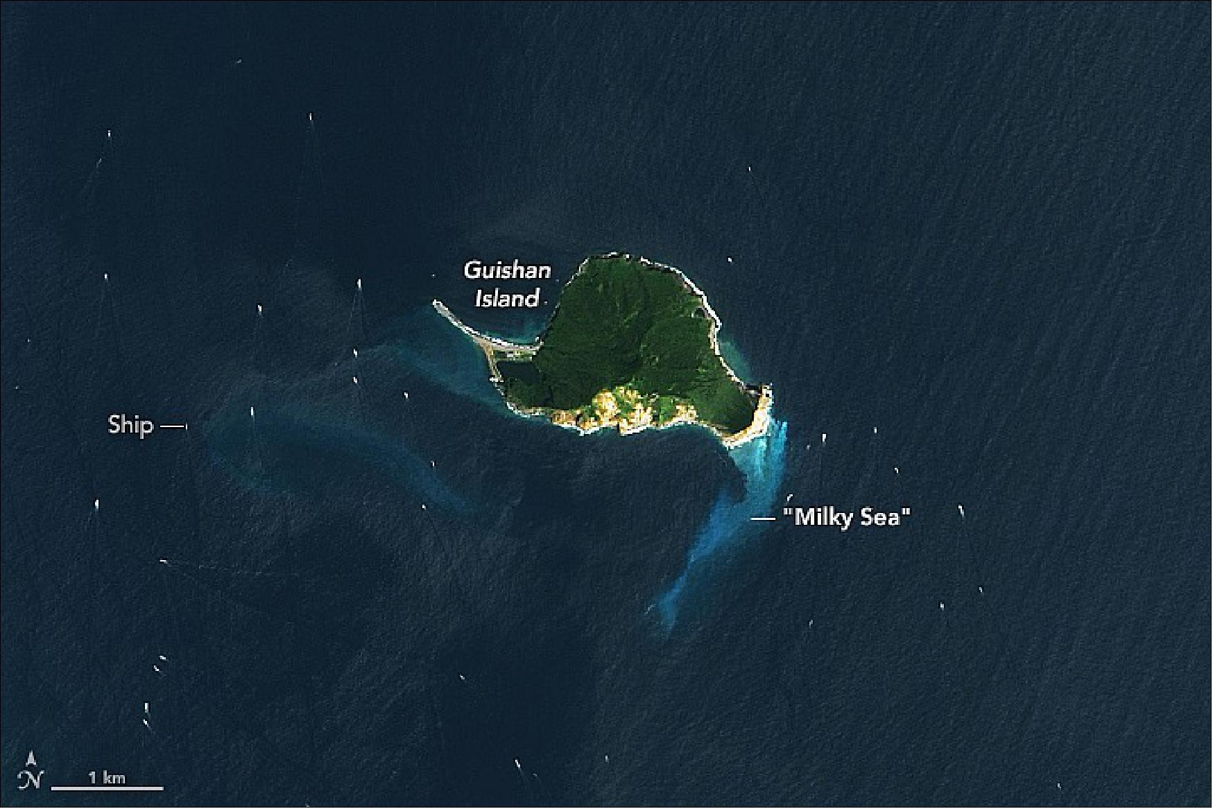
• January 22, 2022: Looking out from the mainland of northeast Taiwan, a turtle-like shape juts above the surface of the Pacific Ocean. Known as Guishan Island, Turtle Island, and Kueishantao, the vegetated rock is the top of a stratovolcano. Its land area spans just under 3 square kilometers (about 1 square mile). 65) The light-blue “Milky Sea” near the "turtle’s head" results from sulfur-rich hydrothermal vents on the seafloor, creating milky water due to sulfur, bacteria, and gas bubbles. Located 5–30m deep, the vents are accessible for study but pose challenges due to hot, acidic, metal-laden water and poor visibility. Research on these vents sheds light on early Earth life and marine ecosystem adaptability. (This is different from the milky sea phenomenon associated with bioluminescence.) In 2016, a 5.8 magnitude earthquake and Typhoon Nepartak caused landslides, blocking vents and altering water chemistry, yet local species adapted. In November 2021, gas plumes were observed, likely due to earthquakes or falling rocks widening vent gaps.
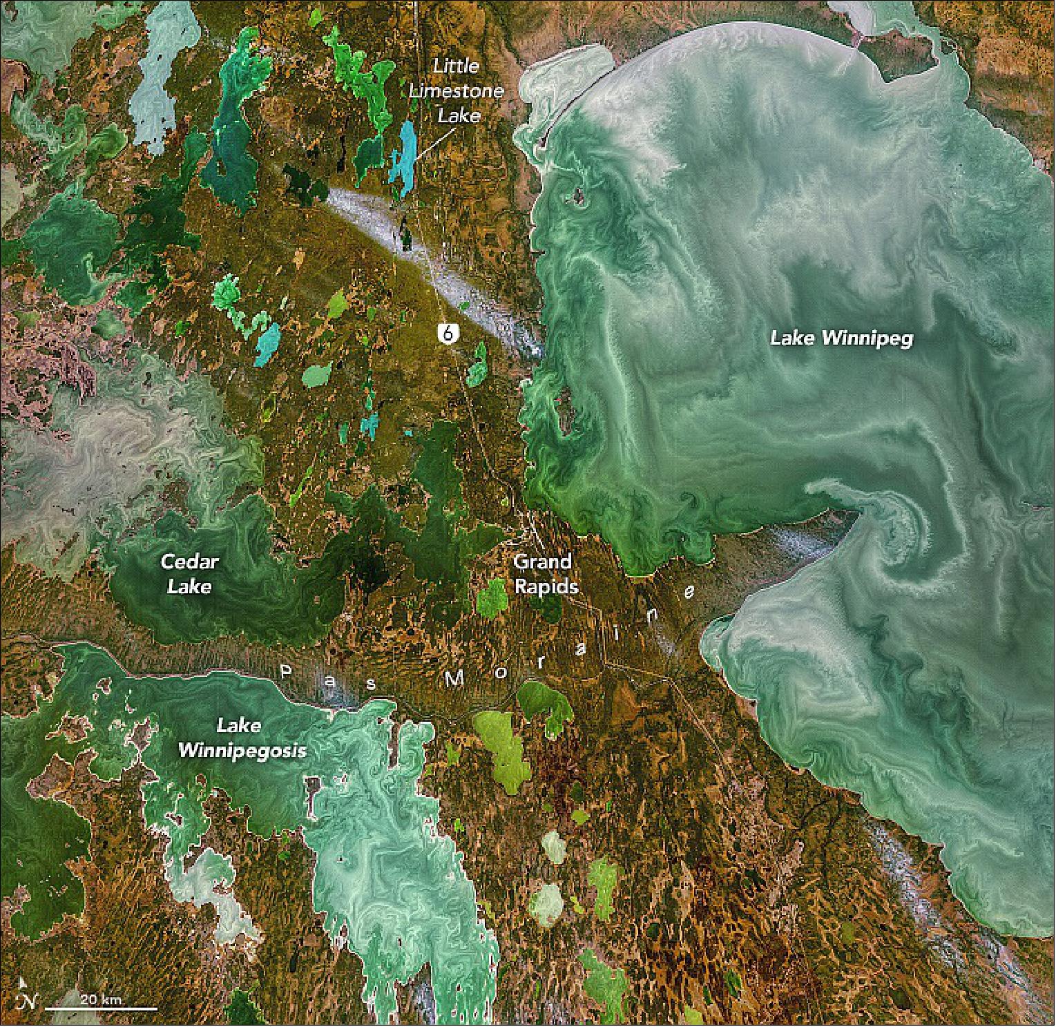
• January 21, 2022: Forty-three percent of the land area of the province of Manitoba, Canada, is covered by bogs, fens, marshes, swamps, and open shallow water. 66) The colourful swirls in the shallow lakes, like Lake Cedar (10m deep), result from suspended sediment and phytoplankton. Fine-grained silt, clay, and calcium-carbonate sediments give some lakes, like Little Limestone Lake, a chalky blue hue. The region's dolomite bedrock, formed in the Paleozoic Era, adds to this effect. The Pas Moraine, the area's most prominent glacial feature, formed when the Laurentide Ice Sheet halted near Cedar Lake, depositing silt, clay, sand, gravel, and rock. When the ice retreated, it left a 300-km (185-mile) crescent-shaped ridge, up to 20 km (12 miles) wide and 30m (100 ft) high, with streamlined ridges and peat-filled swales.
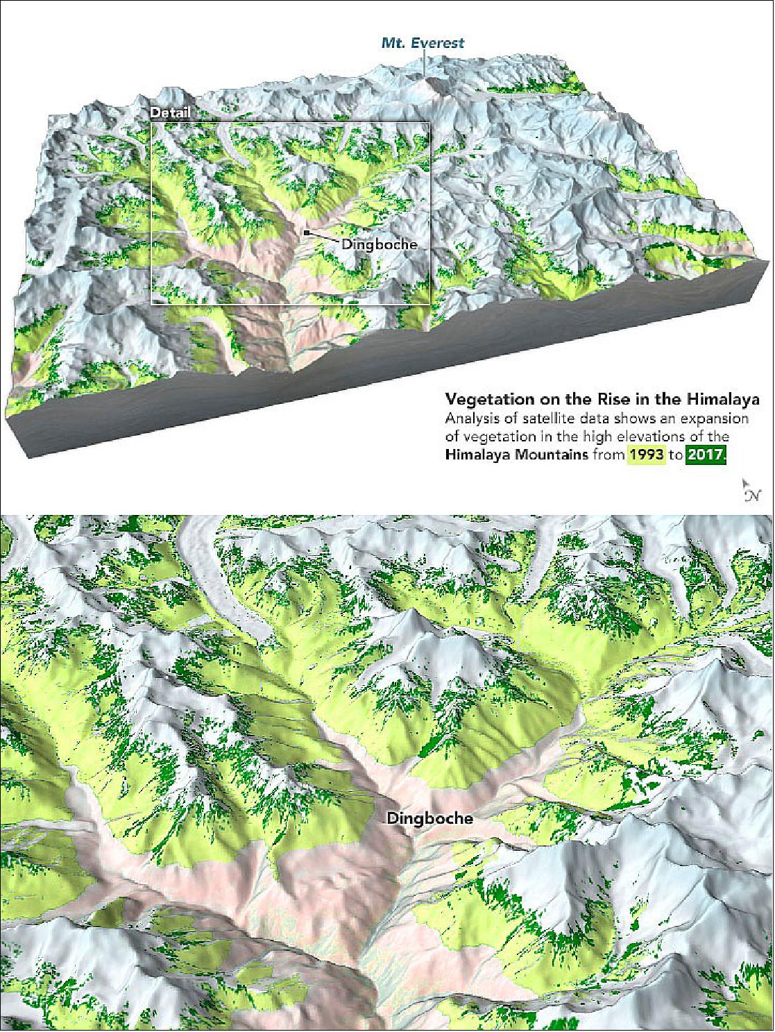
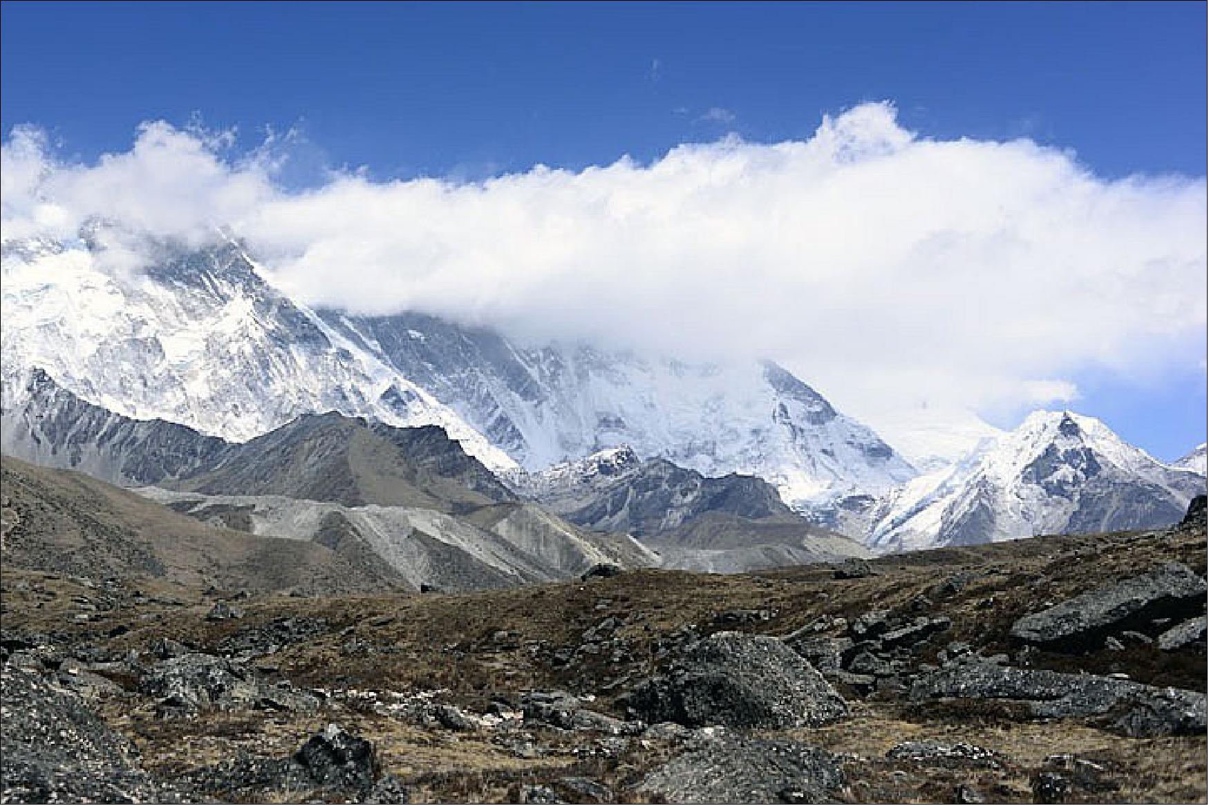
• January 12, 2022: A team led by Karen Anderson, University of Exeter, set out to evaluate how plant life has changed in the Hindu Kush Himalaya over the span of 26 years. They focused on elevations above the tree line but below permanent snow and ice. In this area, known as the subnival or alpine zone, you can find shrubby plants and seasonal snow. In the Himalaya, the zone generally includes altitudes between 4,100 to 6,000 meters (13,000 to 20,000 feet) above sea level. The high altitude and the remoteness of the region add to the challenge of studying its plants. The team used the NDVI ( Normalized Difference Vegetation Index), derived from Landsat satellites. NDVI gives an indication of the land’s greenness, which the scientists used to map the abundance of vegetation across the subnival zone from 1993 to 2018 (using data from Landsat-5, Landsat-7 and Landsat-8). They checked the accuracy of their maps against images from Google Street View and the photographs Anderson shot during her field work in 2017. 67)
• January 10, 2022: Mount Vesuvius, located 12 kilometers (7.5 miles) southeast of Naples, Italy, is the only active volcano on Europe’s mainland. It is a composite stratovolcano, made up of pyroclastic flows, lava flows, and debris from lahars that accumulated to form the volcanic cone. 68) Naples, with 3 million residents, includes 800,000 living on Mount Vesuvius, making it one of the world's most dangerous volcanoes Its A.D. 79 eruption destroyed Pompeii and Herculaneum with deadly pyroclastic flows. Pliny the Younger's eyewitness account of that eruption, including its towering ash cloud, led volcanologists to term these types of eruptions “Vesuvian” or “Plinian.” The threat of such events led to the creation of the first volcanological observatory, in the 19th century. Vesuvius, one of the most studied volcanoes, has had eight eight major eruptions in the past 17,000 years. The most recent, on March 17, 1944, destroyed the village of San Sebastiano, Italy. Since then, the volcano has experienced occasional earthquake activity, ground deformation, and gas venting from the crater.
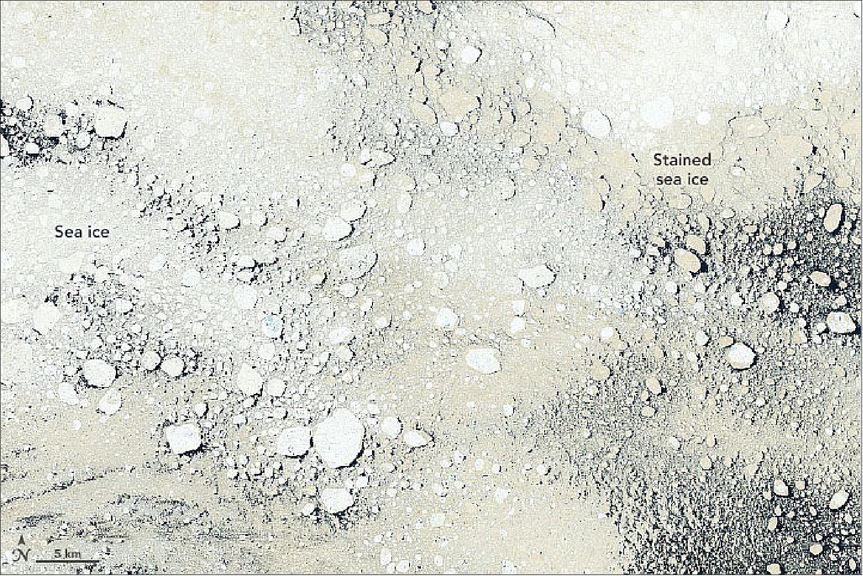
• January 4, 2022: The Foxe basin is known for its 'tan' coloured sea ice. Land surrounds most of the Foxe Basin, so sediment sources are never far away. Since the basin is shallow, winds and waves often stir up sediment from the ocean floor. Particles circulate throughout the water column, sometimes reaching the surface and becoming embedded directly within sea ice. Over time, these sediments can become concentrated in ice at the surface because of sublimation and the melting of the ice. In some areas, the water is shallow enough that sea ice rubs directly against the ocean floor and picks up sediment that way. Some of the colour could also be caused by algae, which can grow under the ice and wash up onto the surface during storms. 69)
• May 30, 2013: NASA transferred operational control of the Landsat-8 satellite to the USGS (U.S. Geological Survey ) in Sioux Falls, S.D, and the mission was officially renamed to Landsat-8. This marks the beginning of the operational phase of the Landsat-8. The USGS now manages the satellite flight operations team within the Mission Operations Center, which remains located at NASA’s Goddard Space Flight Center in Greenbelt, MD. USGS will collect at least 400 Landsat-8 scenes every day from around the world to be processed and archived at the USGS/EROS (Earth Resources Observation and Science Center) in Sioux Falls. 70)
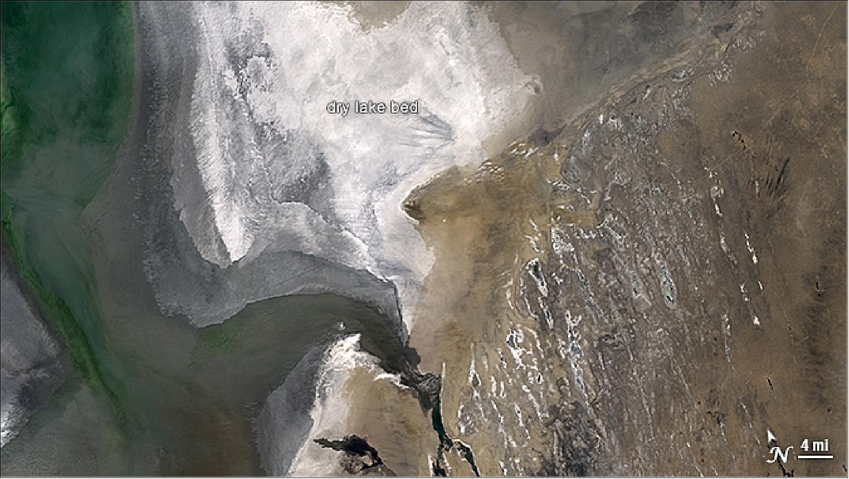
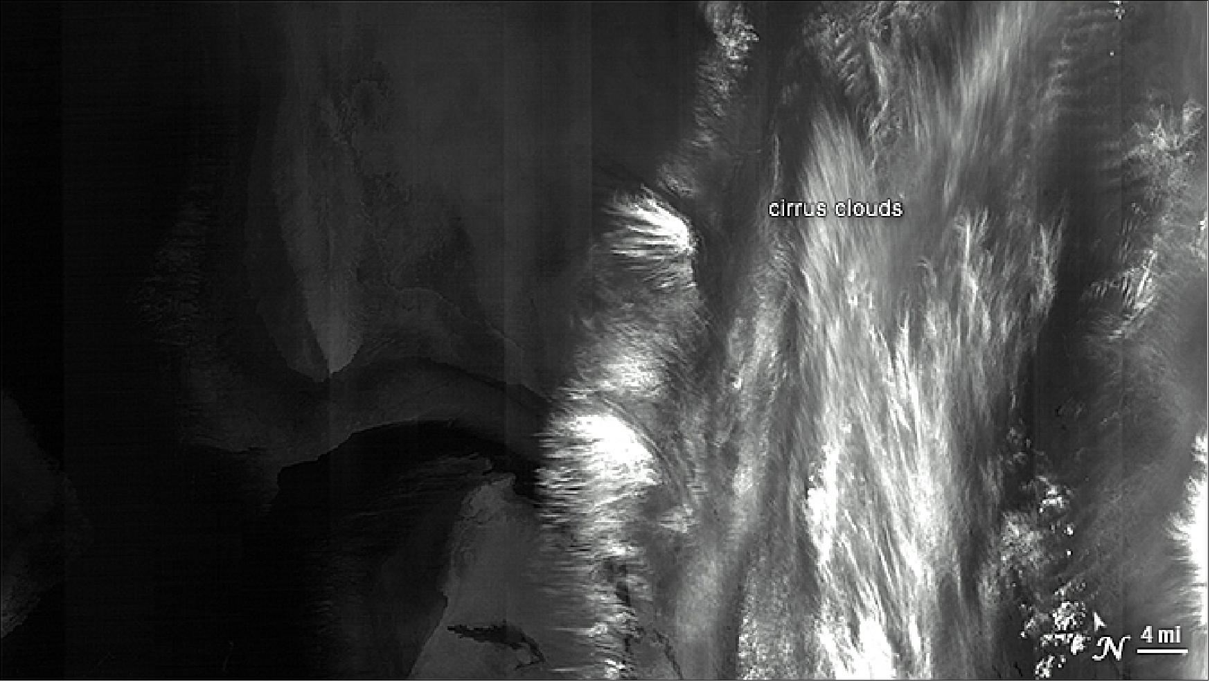
• May 22, 2013: One of two new spectral bands onboard Landsat-8 identifies high-altitude, wispy cirrus clouds that are not apparent in the images from any of the other spectral bands. The March 24, 2013, natural colour image of the Aral Sea, for example, appears to be from a relatively clear day. But when viewed in the cirrus-detecting band, bright white clouds appear. 71) The SWIR band No 9 (1360-1390 nm) is the cirrus detection band of the OLI (Operational Land Imager) instrument. Cirrus clouds are composed of ice crystals. The radiation in this band bounces off of ice crystals of the high altitude clouds, but in the lower regions, the radiation is absorbed by the water vapor in the air closer to the ground. The information in the cirrus band is to alert scientists and other Landsat users to the presence of cirrus clouds, so they know the data in the pixels under the high-altitude clouds could be slightly askew. Scientists could instead use images taken on a cloud-free day, or correct data from the other spectral bands to account for any cirrus clouds detected in the new band. Figures 77 and 78 are simultaneous OLI observations of the same area of the Aral Sea region in Central Asia which illustrate the power of interpretation of a scene. The cirrus clouds of Figure 78 are simply not visible in the natural colour image of Figure 77.
• May 9, 2013: Google released more than a quarter-century of images freely to the public, compiled into an interactive time-lapse experience. Working with data from the Landsat Program, including Landsat-8, the images display a historical perspective on changes to Earth's surface over time. 72) 73) 74) 75)
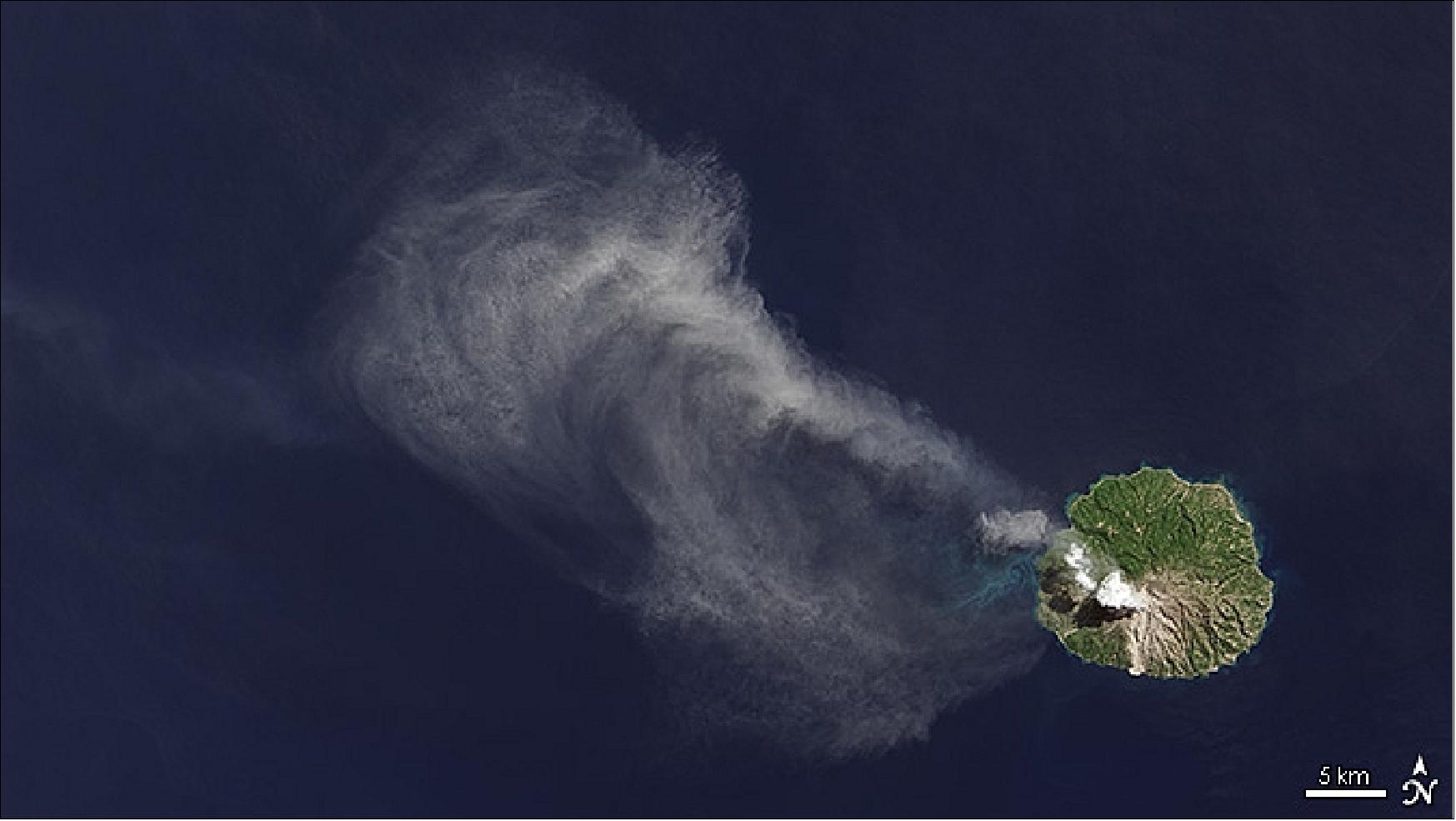
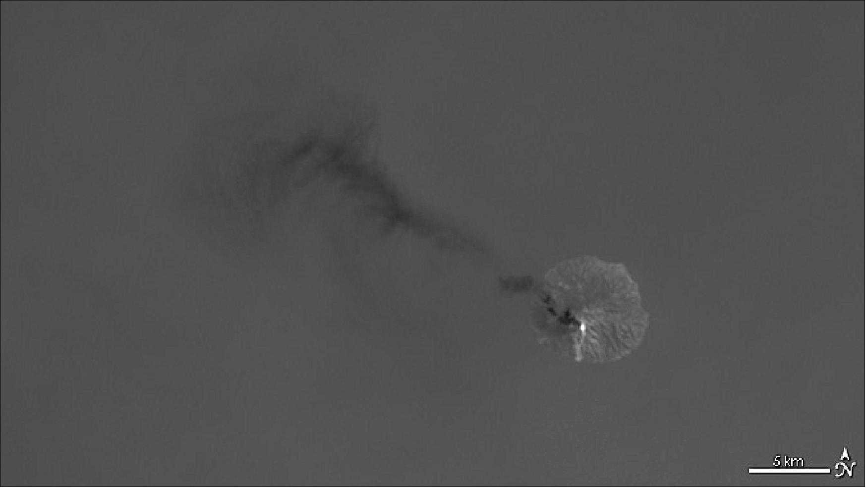
• May 6, 2013: As the LDCM satellite flew over Indonesia's Flores Sea on April 29, it captured an image of Paluweh volcano spewing ash into the air. The satellite's OLI instrument detected the white cloud of smoke and ash drifting northwest over the green forests of the island and the blue waters of the tropical sea. The TIRS (Thermal Infrared Sensor) on LDCM picked up even more. 76) 77) By imaging the heat emanating from the 5-mile-wide volcanic island, TIRS revealed a hot spot at the top of the volcano where lava has been oozing in recent months (Figure 80).
• May 2, 2013: All spacecraft and instrument systems continued to perform normally. LDCM continued to collect more than 400 scenes per day and the U.S. Geological Survey Data Processing and Archive System continued to test its ability to process the data flow while waiting for the validation and delivery of on-orbit calibration, which convert raw data into reliable data products. 78)
• April 12, 2013: LDCM (Landsat Data Continuity Mission) reached its final altitude of 705 km. One week later, the satellite’s natural-colour imager (OLI) scanned a swath of land 185 km wide and 9,000 km long. 79) 80)
• April 4, 2013: LDCM was on WRS-2 (Worldwide Reference System-2).
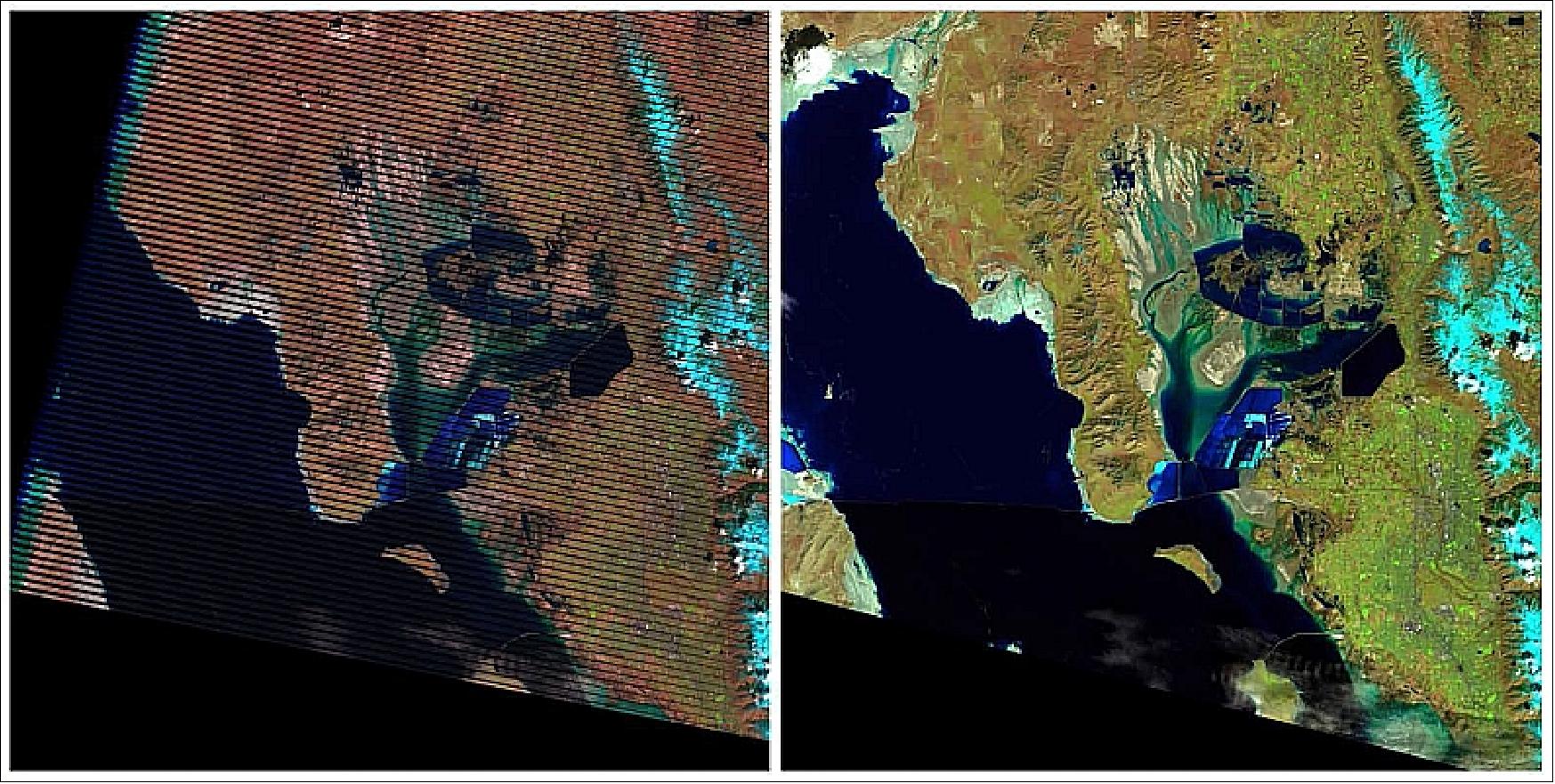
• March 21, 2013: Since launch, LDCM had been going through on-orbit testing. The mission operations team completed its review of all major spacecraft and instrument subsystems, and performed multiple spacecraft attitude maneuvers to verify the ability to accurately point the instruments. 82) As planned, LDCM was flying in an orbit slightly lower than its operational orbit of 705 km above Earth's surface. As the spacecraft's thrusters raised its orbit, the NASA-USGS team took the opportunity to collect imagery while LDCM was flying under Landsat 7, also operating in orbit. Measurements collected simultaneously from both satellites allowed the team to cross-calibrate the LDCM sensors with Landsat 7's Enhanced Thematic Mapper-Plus instrument.
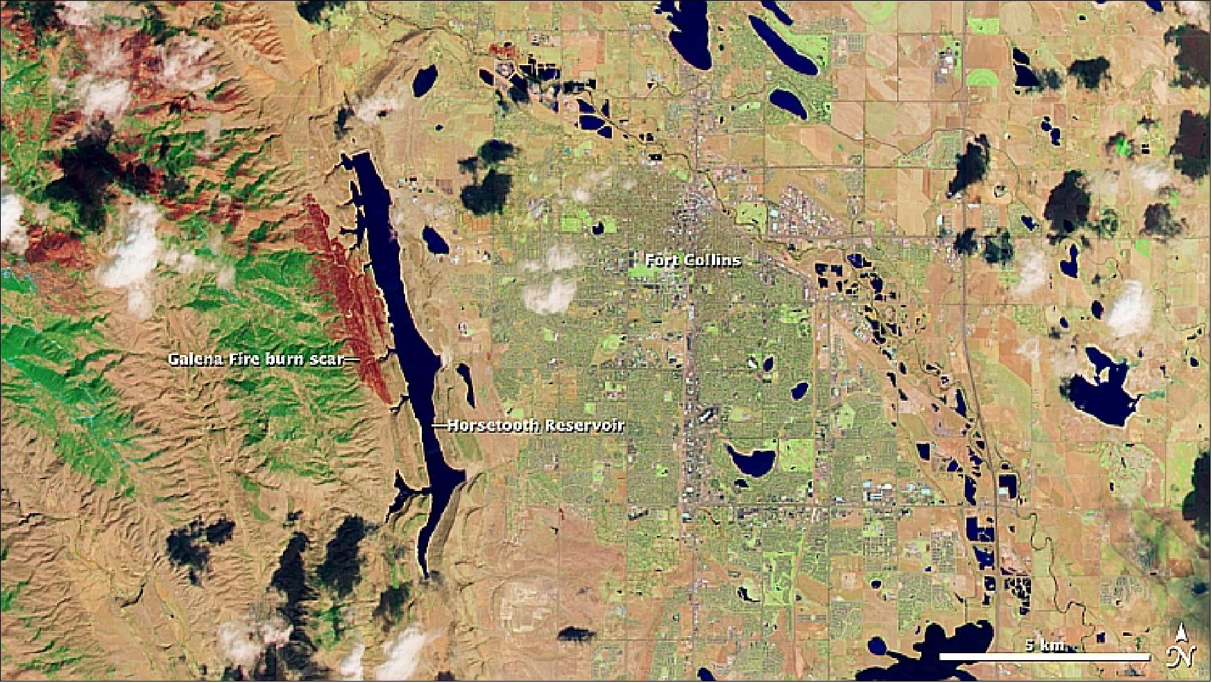
• March 18, 2013: First day of simultaneous OLI and TIRS Earth imaging (Ref. 80).
• February 21, 2013: The LDCM mission operations team successfully completed the first phase of spacecraft activation. All spacecraft subsystems were turned on, including propulsion, and power was supplied to the OLI (Operational Land Imager) and TIRS (Thermal Infrared Sensor) instruments. 84)
• February 11, 2013: The LDCM spacecraft separated from the rocket 79 minutes after launch and the first signal was received 3 minutes later at the ground station in Svalbard, Norway. The solar arrays deployed 86 minutes after launch, and the spacecraft started generating power from them (Ref. 25). LDCM went through a check-out phase for the next three months. Afterward, operational control was transferred to NASA's mission partner, the USGS (U.S. Geological Survey), and the satellite renamed to Landsat-8. The data was archived and distributed free over the Internet from the EROS (Earth Resources Observation and Science) center in Sioux Falls, S.D. Distribution of Landsat-8 data from the USGS archive was expected to begin within 100 days of launch.
Sensor Complement
Background: In 2008 the TIRS (Thermal Infrared Sensor) instrument was still regarded an option to the LDCM mission. However, in Dec. 2009, the US government confirmed that TIRS would be developed and would be on board the LDCM spacecraft. In the spring of 2010, TIRS passed the CDR (Critical Design Review). 85) 86)
The OLI and TIRS data are merged into a single data stream. Together the OLI and TIRS instruments on LDCM replace the ETM+ instrument on Landsat-7 with significant enhancements.
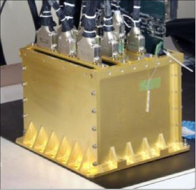
OLI (Operational Land Imager)
Already in July 2007, NASA had awarded a contract to BATC (Ball Aerospace Technology Corporation) of Boulder, CO, to develop the OLI (Operational Land Imager) key instrument for LDCM. The BATC contract terms call for the design, development, fabrication and integration of one OLI flight model. Furthermore, the company is also required to test, deliver and provide post-delivery support and five years of on-orbit support for the instrument.
The multispectral and moderate resolution OLI instrument has similar spectral bands to the ETM+ (Enhanced Thermal Mapper plus) sensor of Landsat-7. It includes new coastal aerosol (443 nm, band 1) and cirrus detection (1375 nm, band 9) bands, though it does not have a thermal infrared band.
The following list provides an overview of the most important observation requirements for the OLI instrument: 87)
• The specifications require delivery of data covering at least 400 Landsat scenes/day (185 km x 180 km) for the US archive. The data are to be acquired in a manner that affords seasonal coverage of the global land mass. Data are required for the heritage reflective Thematic Mapper (TM) spectral bands plus two new bands, a blue band for coastal zone observations and a short wave infrared band for cirrus cloud detection.
• 30 m GSD (Ground Sample Distance) for VIS/NIR/SWIR, 15m GSD for PAN data.
• The specifications do not require thermal data (TIR band), representing a departure from the TM (Thematic Mapper) heritage. The specification also requires data providing a 30 m GSD (Ground Sample Distance) for each of the multispectral bands. Note: The TIR band was deselected due to the extra cost of active cooling.
• An edge response slope is also specified for the image data from each spectral band. The edge response is defined as the normalised response of the image data to a sharp edge as expressed in a Level 1R VDP (Validation Data Product). An edge response slope of 0.027 is required for bands 1 through 7, a slope of 0.054 is required for the panchromatic band, band 8, and a slope of 0.006 for the cirrus band, band 9.
• All instrument source data will be quantized to 12 bit resolution.
Band Nr | Band Name | Spectral range (nm) | Use of data | GSD | Radiance (W/m2 sr μm), typical | SNR |
1 | New Deep Blue | 433-453 | Aerosol/coastal zone | 30 m | 40 | 130 |
2 | Blue | 450-515 | Pigments/scatter/coastal |
30 m | 40 | 130 |
3 | Green | 525-600 | Pigments/coastal | 30 | 100 | |
4 | Red | 630-680 | Pigments/coastal | 22 | 90 | |
5 | NIR | 845-885 | Foliage/coastal | 14 | 90 | |
6 | SWIR 2 | 1560-1660 | Foliage | 4.0 | 100 | |
7 | SWIR 3 | 2100-2300 | Minerals/litter/no scatter | 1.7 | 100 | |
8 | PAN | 500-680 | Image sharpening | 15 m | 23 | 80 |
9 | SWIR | 1360-1390 | Cirrus cloud detection | 30 m | 6.0 | 130 |
• The WRS-2 (Worldwide Reference System-2) defines Landsat scenes as 185 km x 180 km rectangular areas on the Earth's surface designated by path and row coordinates. This heritage system is used to catalogue the data acquired by the Landsat 4, 5, and 7 satellites and will also be used for the LDCM.
• Provide “standard”, orthorectified data products within 24 hours of observation (products available via the web at no cost)
• Data calibration consistent with previous Landsat missions
• Continue IC (International Cooperator) downlinks
• Support priority imaging and a limited off-nadir collection capability (± 1 path/row).
OLI (LDCM) | ETM+ (Landsat-7) | ||||
Band Nr | Wavelength (µm) | GSD (m) | Band No. | Wavelength (µm) | GSD (m) |
8 (PAN) | 0.500 - 0.680 | 15 | 8 (PAN) | 0.52 - 0.90 | 15 |
1 | 0.433 - 0.453 | 30 |
|
|
|
2 | 0.450 - 0.515 | 30 | 1 | 0.45 - 0.52 | 30 |
3 | 0.525 - 0.600 | 30 | 2 | 0.53 - 0.61 | 30 |
4 | 0.630 - 0.680 | 30 | 3 | 0.63 - 0.69 | 30 |
|
|
| 4 | 0.78 - 0.90 | 30 |
5 | 0.845 - 0.885 | 30 |
|
|
|
9 | 1.360 - 1.390 | 30 |
|
|
|
6 | 1.560 - 1.660 | 30 | 5 | 1.55 - 1.75 | 30 |
7 | 2.100 - 2.300 | 30 | 7 | 2.09 - 2.35 | 30 |
OLI does not include thermal imaging capabilities | 6 (TIR) | 10.40 - 12.50 | 60 | ||
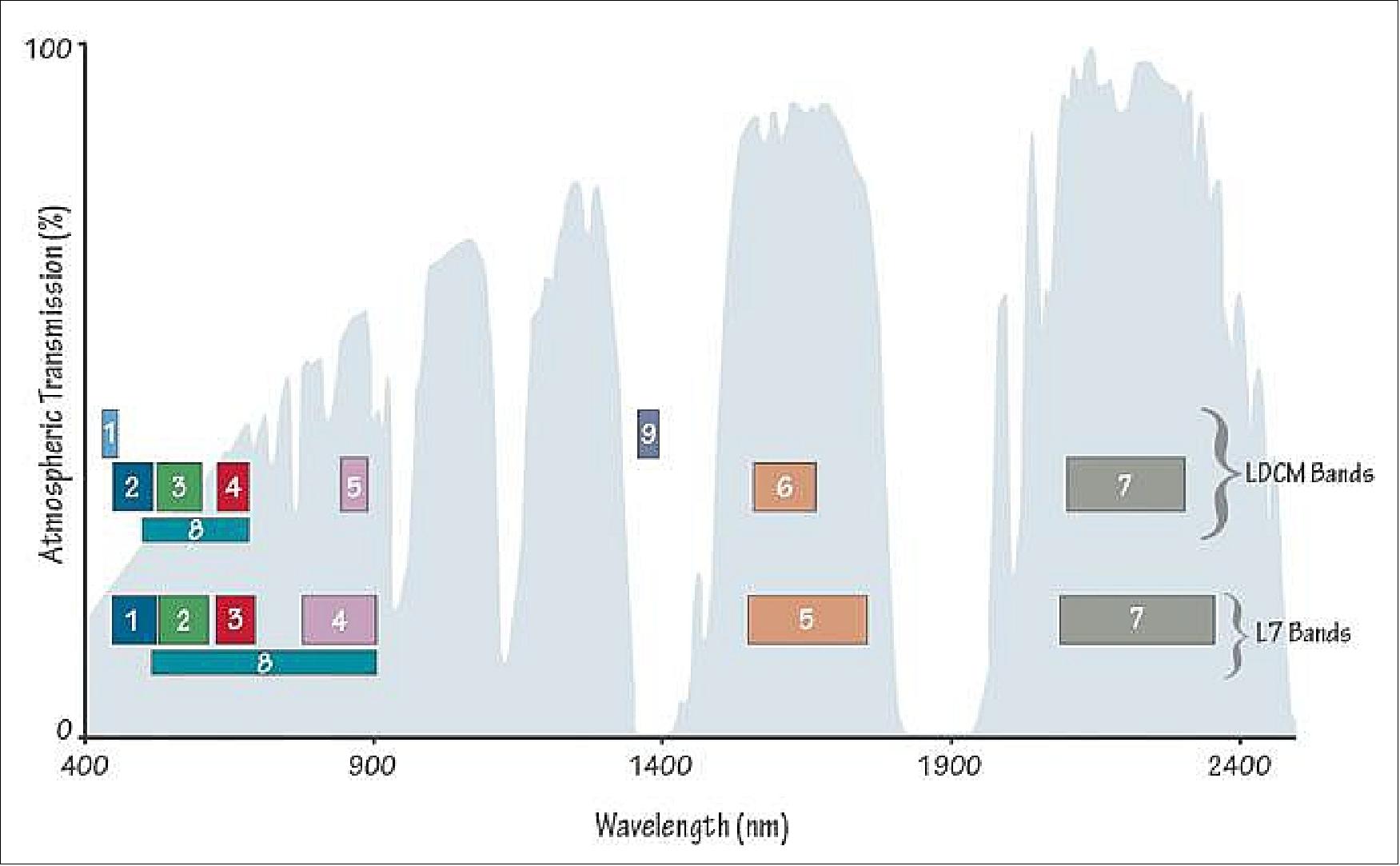
OLI Instrument
The OLI design features a multispectral imager with a pushbroom architecture (Figure 86) of ALI (Advanced Land Imager) heritage, a technology demonstration instrument flown on the EO-1 spacecraft of NASA (launch Nov. 21, 2000). A pushbroom implementation is considered to be more geometrically stable than the whiskbroom scanner of the ETM+ instrument. As a tradeoff of this architecture selection, the imagery must be terrain corrected to ensure accurate band registration.. 88) 89) 90) 91) 92)
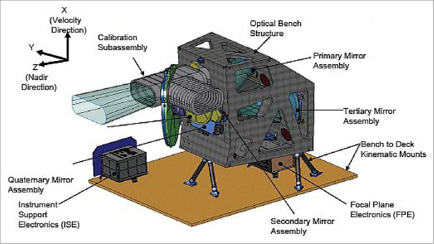
The FPA (Focal Plane Assembly) consists of 14 FPMs (Focal Plane Modules). This is a consequence of the pushbroom architecture selection for OLI leading to a different set of geometric challenges than a cross-track whiskbroom implementation. Instead of using a small focal plane and a scanning mirror, 14 FPMs are required to cover the full Landsat cross-track field of view. Each FPM contains nine spectral bands in along-track (Figure 87). The along-track spectral band separation leads to an approximately 0.96-second time delay between the leading and trailing bands. This time delay creates a small but significant terrain parallax effect between spectral bands, making band registration more challenging.
The along-track dimension of the OLI focal plane (see Figure 88) also makes it desirable to “yaw steer” the spacecraft. This means that the spacecraft flight axis is aligned with the ground (Earth fixed) velocity vector, rather than with the inertial velocity vector, in order to compensate for cross-track image motion due to Earth rotation.
Although the pushbroom architecture requires many more detectors and a correspondingly larger focal plane, it also allows for a much longer detector dwell time (~4 ms for OLI vs. 9.6 µs for ETM+), leading to much higher signal-to-noise ratios. The lack of moving parts in the pushbroom design also allows for a more stable imaging platform and good internal image geometry.
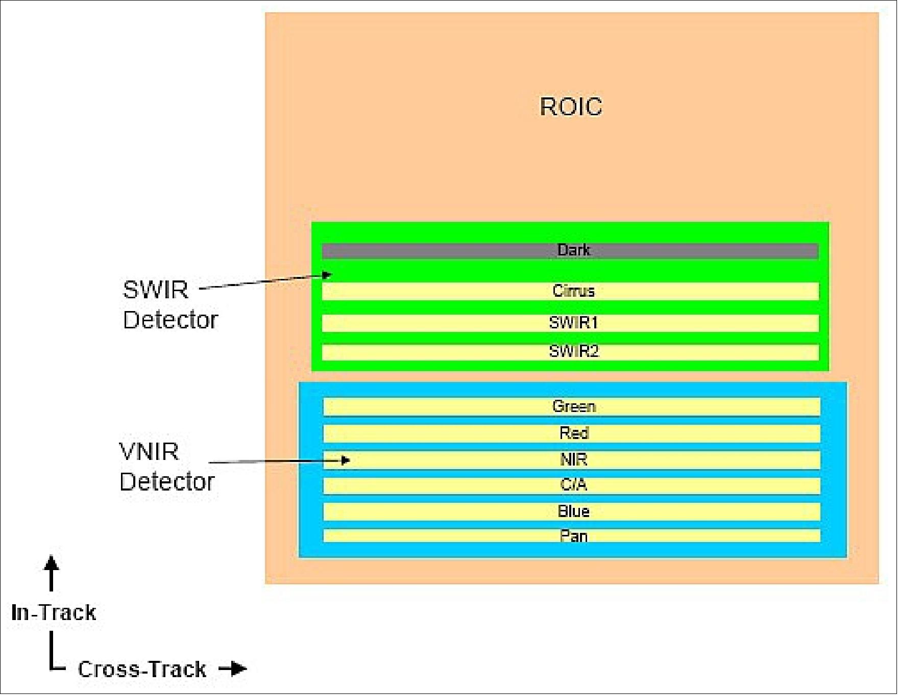

Each FPM contains detectors for each spectral band, silicon for the VNIR bands and HgCdTe for the SWIR bands and a butcher-block filter assembly to provide the spectral bands.
OLI features about 6500 active detectors per multispectral band and 13000 detectors for the panchromatic band. These detectors are organized as blocks ~500 multispectral (1000 panchromatic) detectors wide within 14 focal plane modules (FPMs) that make up the focal plane assembly. Each module has its own butcher-block assembly spectral filter. This provides significantly improved signal to noise performance, but complicates the process of radiometrically matching the detectors responses. Similarly, the lack of a scan mirror removes the need for knowledge of its movement, but requires knowledge of the detectors locations across a much larger focal plane (Ref. 2).
Observation technique | Pushbroom imager |
Spectral bands | 9 bands in VNIR/SWIR covering a spectral range from 443 nm to 2300 nm |
Telescope | - Four-mirror off-axis telescope design with a front aperture stop |
FPA (Focal Plane Assembly) | - Consisting of 14 sensor chip assemblies mounted on a single plate |
Swath width (FOV=15º) | 185 km |
GSD (Ground Sample Distance) | 15 m for PAN data; 30 m for VNIR/SWIR multispectral data |
Data quantization | 12 bit |
Calibration | - Solar calibrator (diffuser) used once/week |
Instrument, mass, power, size |
|
The OLI will provide global coverage by acquiring ~400 scenes per day in six VNIR and three SWIR bands, all at 12 bit radiometric resolution. In addition to these bands, there will be a tenth band consisting of covered SWIR detectors, referred to as the ‘blind’ band, that will be used to estimate variation in detector bias during nominal Earth image acquisitions. The OLI bands are distributed over 14 SCAs (Sensor Chip Assemblies) or FPMs, each with 494 detectors per 30 m band and twice as many for the 15 m panchromatic band - totaling in over 75000 imaging detectors. 93)
OLI Calibration
The OLI calibration subsystem (Figures 89 and 90) consists of two solar diffusers (a working and a pristine), and a shutter. When positioned so that the sun enters the solar lightshade, the diffusers reflect light diffusely into the instruments aperture and provide a full system full aperture calibration. The shutter, when closed, provides a dark reference. In addition, two stim lamp assemblies are located at the front aperture stop. Each lamp assembly contains three lamps (per redundant configuration) that are operated at constant current and monitored by a silicon photodiode. The lamp signal goes through the full telescope system. Additionally, the OLI focal plane will include masked HgCdTe detectors, that is, detectors that will be blocked from seeing the Earth’s radiance (Ref. 2). 94) 95)
• Solar diffusers:
- Full-aperture full system Spectralon diffuser, designed to be used at different frequencies to aid in tracking the system and diffuser changes. The pristine diffuser will be used to check degradation of main diffuser.
- The primary solar diffuser will nominally be deployed every 8 days to track the calibration of the OLI sensor and perform detector-to-detector normalization.
- The solar diffuser based calibration requires a spacecraft maneuver to point the OLI solar calibration aperture towards the sun. The pristine diffuser will be used on a less frequent basis, about every six months, as a check on the primary diffuser's degradation.
• Stimulation lamps:
- Multi—bulbed tungsten lamp assemblies, that illuminate the OLI detectors through the full optical system, similarly designed to be used at different frequencies to separate lamp and system changes. The working lamp will be used daily for intra-orbit calibration/characterization; the reference lamp set approximately monthly, and the pristine lamp set approximately twice a year.
- The lamb assembly can also be compared to solar diffuser measurements to check stability.
• Dark shutter:
- Used twice per orbit for offset calibration
• Dark detectors on focal plane to monitor offset drift
• Linearity checked by varying detector integration time.
The LDCM operational concept also calls for the spacecraft to be maneuvered every lunar cycle to view the moon, providing a "known" stable source for tracking stability over the mission. A side-slither maneuver, where the spacecraft is rotated 90º to align the detector rows with the velocity vector, is also planned. These data will provide an additional method to assess the detector-to-detector radiometric normalization.
Pre-launch spectro-radiometric characterization and calibration (Ref. 94):
The spectral characterization of the OLI instrument is being performed at the component, focal plane module and fill instrument levels. The components, which have all completed testing, include detector witness samples, spectral filters prior to dicing into flight filter sticks, the focal plane assembly window witness samples and telescope mirror witness samples.
The FPM (Focal Plane Module) level tests, which are also complete, are specifically designed to characterize the spectral out-of-band response. The FPM level tests measure the spectral response of all the detectors by illuminating the full focal plane at approximately the correct cone angle.
An integrating sphere is used in the pre-launch radiance calibration of the OLI. The traceability of the calibration of this sphere will start with the 11" OLI transfer sphere directly calibrated at the NIST Facility for Spectroradiometric Calibration (FASCAL). While still at NIST, this OLI transfer sphere is checked by independently NIST calibrated University of Arizona (UAR VNIR transfer radiometer), NASA and NIST (Government Transfer Radiometers) radiometers. Also, the Ball Standard Radiometer (BSR), that has filters matching the OLI bands, views the sphere.
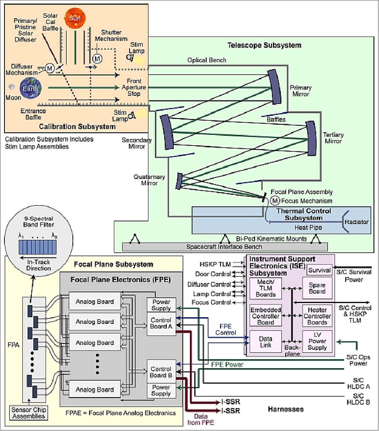
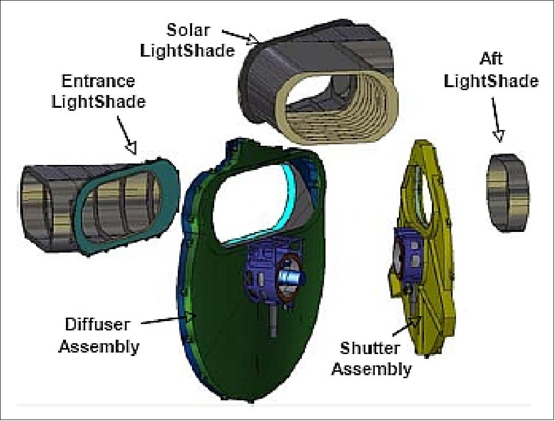
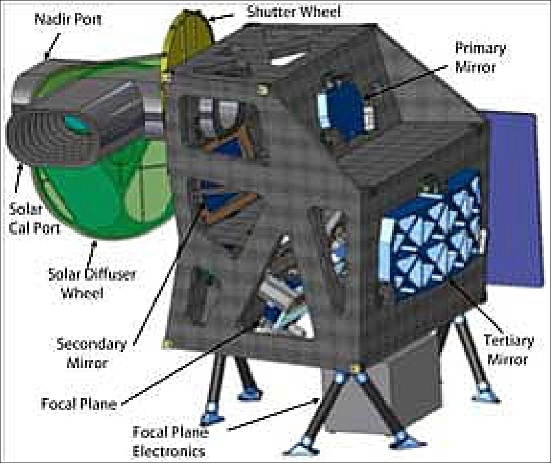
In Nov. 2008, the OLI instrument passed the ICDR (Instrument Critical Design Review). 96)
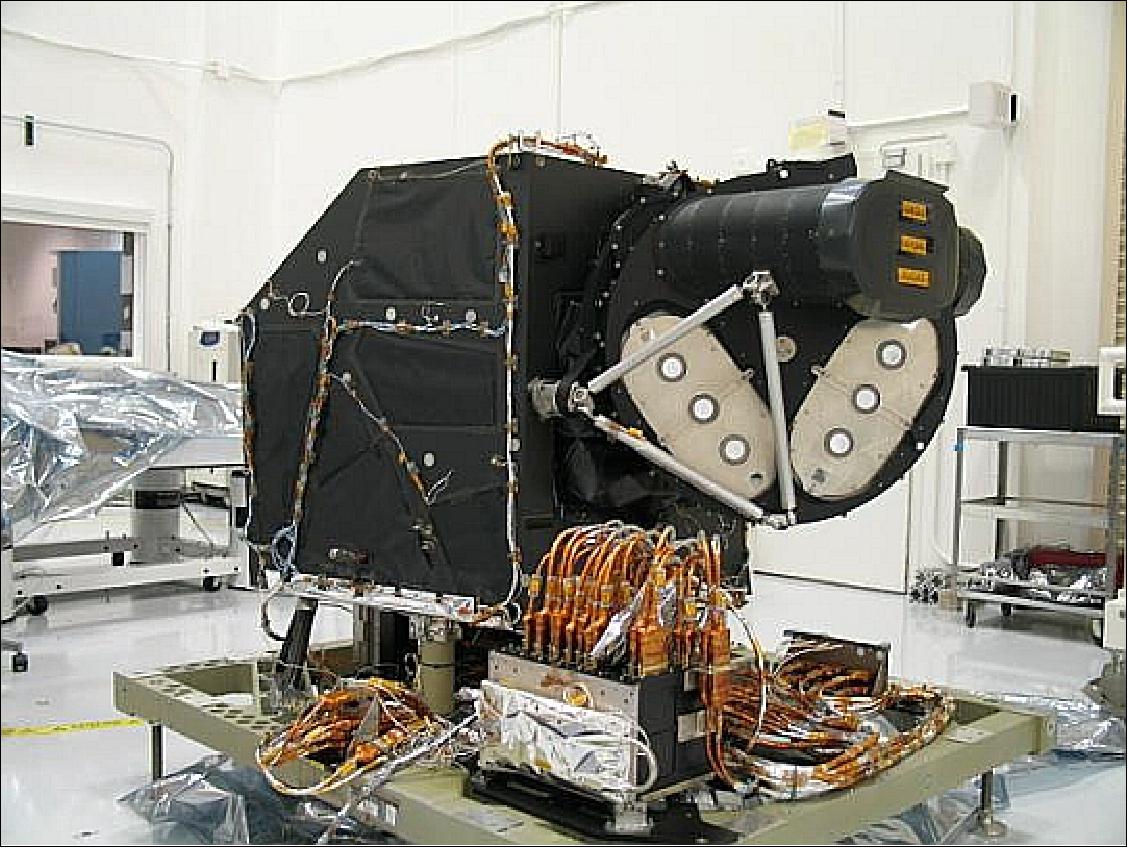
Delivery of the OLI instrument in the summer of 2011 (Ref. 3).
TIRS (Thermal Infrared Sensor)
The TIRS instrument is providing continuity for two infrared bands not imaged by OLI. NASA/GSFC is building the TIRS instrument inhouse. TIRS is a late addition to the LDCM mission, the requirements call for a GSD (Ground Sample Distance of 120 m for the imagery; however, the actual GSD will be 100 m.
The LDCM ground system will merge the data from both sensors into a single multispectral image product. These data products will be available for free to the general public from the USGS enabling a broad scope of scientific research and land management applications. 97) 98)
TIRS is a QWIP (Quantum Well Infrared Photodetector) based instrument intended to supplement the observations of the OLI instrument. The TIRS instrument is a TIR (Thermal Infrared) imager operating in the pushbroom mode with two IR channels: 10.8 µm and 12 µm. The two spectral bands are achieved through interference filters that cover the FPA (Focal Plane Assembly). The pushbroom implementation increases the system sensitivity by allowing longer integration times than whiskbroom sensors. The two channels allow the use of the “split-window” technique to aid in atmospheric correction.
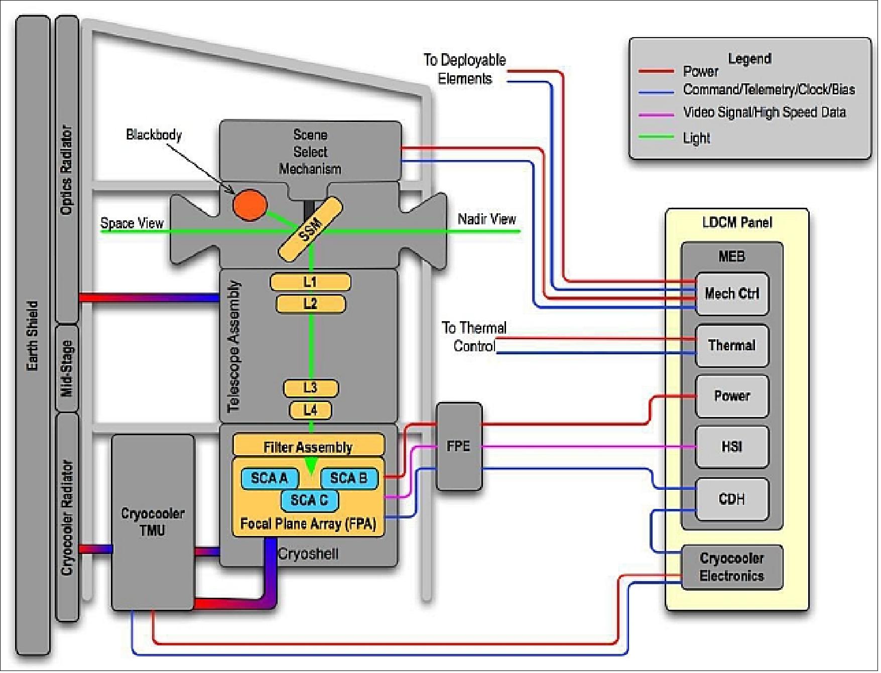
The focal plane consists of three 640 x 512 QWIP GaAs arrays mounted on a silicon substrate that is mounted on an invar baseplate. The two spectral bands are defined by bandpass filters mounted in close proximity to the detector surfaces. The QWIP arrays are hybridized to ISC9803 readout integrated circuits (ROICs) of Indigo Corporation. The focal plane operating temperature will be maintained at 43 K (nominally). 99) 100) 101)
Instrument type | Pushbroom imager |
Two channel thermal imaging instrument | 10.8 and 12.0 µm band centers |
Bandwidths | 10.3-11.3 µm, |
GSD (Ground Sample Distance) | 100 m (nominal), 120 m (requirement) |
Swath width | 185 km, FOV = 15º |
Operating cadence | 70 frames/s |
Instrument calibration | - Scene select mirror to select between 2 calibration sources |
Detector | - Three SCA (Sub-Chip Assembly) QWIP detectors built in-house at Goddard |
Telescope | - The telescope is a 4-element refractive lens system. |
Telescope f number | f/1.64 |
Data quantization | 12 bit |
Instrument mass, size, power | 236 kg, approx: 80 cm x 76 cm x 43 cm, 380 W |
QWIP detector: The development of the QWIP detector technology has made great strides in the first decade of the 21st century. In 2008, NASA/GSFC revised the design of the infrared detector concept of the TIRS (Thermal Infrared Sensor) imager, under development for the LDCM (Landsat Data Continuity Mission). The initially considered HgCdTe-based detector design was changed to a QWIP design due to the emergence of broadband QWIP capabilities in the MWIR and TIR (LWIR) regions of the spectrum. The introduction of QWIP technology for an operational EO mission represents a breakthrough made possible through collaborative efforts of GSFC, the Army Research Lab and industry (Ref. 100).
An important advantage of GaAs QWIP technology is the ability to fabricate arrays in a fashion similar to and compatible with the silicon IC technology. The designer’s ability to easily select the spectral response of the material from 3 µm to beyond 15 µm is the result of the success of band-gap engineering. 102)
Advantages of QWIP technology:
- Large lattice-matched substrates
- Mature materials technology
- No unstable mid-gap traps
- Inherently, radiation hard.
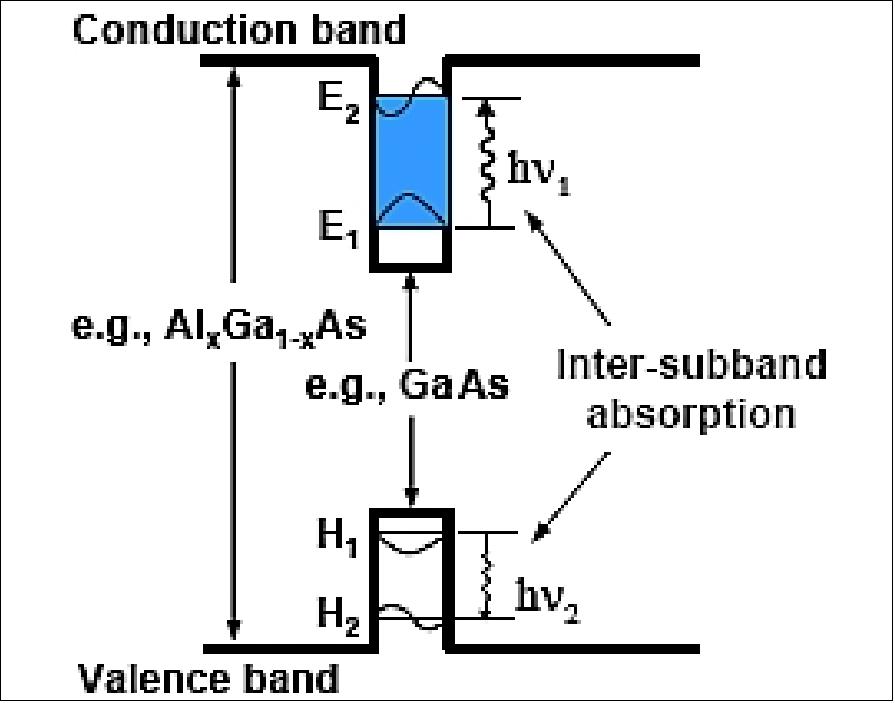
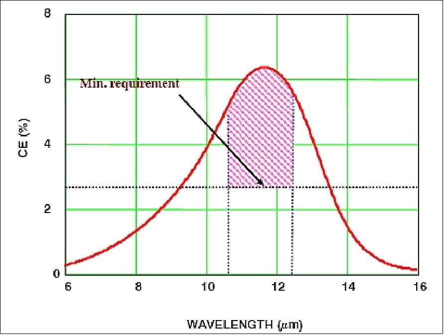
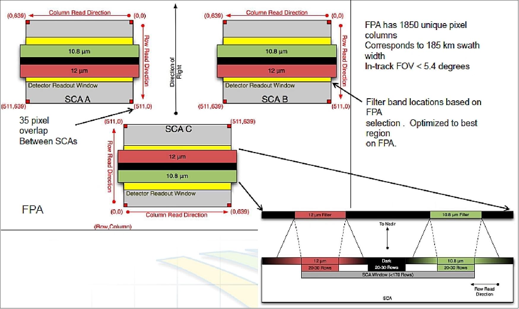
The three arrays are precisely aligned to each other in the horizontal and vertical directions (to within 2 µm). There is a requirement that the detection region within the QWIP array be within 10 µm of a common focal plane altitude. This specification is challenging since it includes surface non-uniformities of the baseplate, substrate, the QWIP/ROIC hybrid and the epoxy bond lines between these components. Nonetheless, since there are three discreet arrays they must all fall within a single focus position.
The filter bands are further confined to specific regions of the QWIP array. Although each array contains 512 rows, after all the operational requirements are satisfied (frame rate, windowing, co-registration, scene reconstruction, etc.) only 32 rows are available under each filter band separated by 76 rows of occluded pixels (for dark current subtraction). Once all these requirements are incorporated into the focal plane design, eligible rows on any given array are pre-determined. Of these eligible rows, there must be three that can be combined to make two perfect rows, or preferably, at least two perfect rows (that is, rows where all pixels meet every specification).
TRL (Technology Readiness Level) tests: An important and essential process for qualifying new or previously unused technology in a NASA space mission is the technology readiness level demonstration. There are nine levels with level 6 (TRL 6) being the level at which new hardware must be demonstrated. Typically, this means qualification in the environment which the instrument will be subjected through out the mission; radiation effects, vibration, thermal cycling and (in some cases) shock. Both the readout and QWIP hybrids were subjected to gamma, proton and heavy ion radiation equivalent to 35 krad or almost 10 times the expected mission dose. At these levels and at the operating temperature of 43 K minimal effects were observed and none were considered to be a mission risk.
A fully functioning focal plane assembly was subjected to 40 thermal cycles from 300 K to 77 K and back to 300 K. Every tenth cycle went to 43 K to collect the array performance data. After the completion of the 40 cycles there was essentially no change in any of the three QWIP arrays (2 grating QWIP hybrids and one C-QWIP hybrid). - The final environmental test performed was vibration to simulate the effect of the launch. Since this is a qualification test the vibration loads are specified 3db above the expected loads. The focal plane assembly was subjected to a series of vibration input loads including x, y and z-axis random vibration for 2 minutes/axis, a sine sweep and sine burst test (15 g at 20 Hz). No failures occurred and this assembly and the overall design was certified by an independent review panel as having met the requirements for TRL 6.


Legend to Figure 98: The left photo of the FPA is without filters showing the 3 QWIPs in the center. The daughter boards are the red and green assemblies to the left and right, respectively. The invar spider is the component with the 4 arms. - The right picture of the FPA comes with the filters attached. Note that there are two filters over each array with a thin dark strip between them.
Optical system: The imaging telescope is a 4-element refractive lens system. A scene select mechanism (SSM) rotates a scene mirror (SM) to change the field of regard from a nadir Earth view to either an on-board blackbody calibrator or a deep space view. The blackbody is a full aperture calibrator whose temperature may be varied from 270 to 330 K.
The optical system, consisting of a lens with three Ge elements and one ZnSe element, produces nearly diffraction-limited images at the focal plane. All but 2 of the surfaces are spherical, which simplifies fabrication. The optics are radiatively cooled to a nominal temperature of 185 K to reduce the contribution of background thermal emission to the measurement noise. Because of the fairly strong thermal dependence of the index of refraction of Ge, the focus position of the lens is a function of the optics temperature. This provides a method of adjusting focus so that, in the unlikely event that launch conditions or some other effect defocus the system, the temperature of the optics may be changed by ±5 K to refocus. That is, thermal control of the lens provides a non-mechanical focus mechanism. A +5 K change does not significantly degrade the noise performance.
A precision scene select mirror is an essential component of the TIRS instrument and it is driven by the scene select mechanism. It rotates around the optical axis on a 45º plane to provide the telescope with a view of Earth through the nadir baffle and two full aperture sources of calibration, onboard variable temperature blackbody (hot calibration target) and space view (cold calibration target). The onboard blackbody will be a NIST (National Institute of Standards and Technology) certified reference source (Figure 99).
TIRS is able to achieve a 185 km ground swath with a 15º FOV (Field of View) functioning in the pushbroom sample collection method. This method will have the benefit of being able to collect and record data without movement artifacts due to its wide instantaneous field of view. Frames will be collected at an operating cadence of 70 per second. The collected data will be stored temporarily stored on board and periodically sent to the USGS EROS facility for further storage. The instrument is designed to have an expected lifetime of at least a three years.
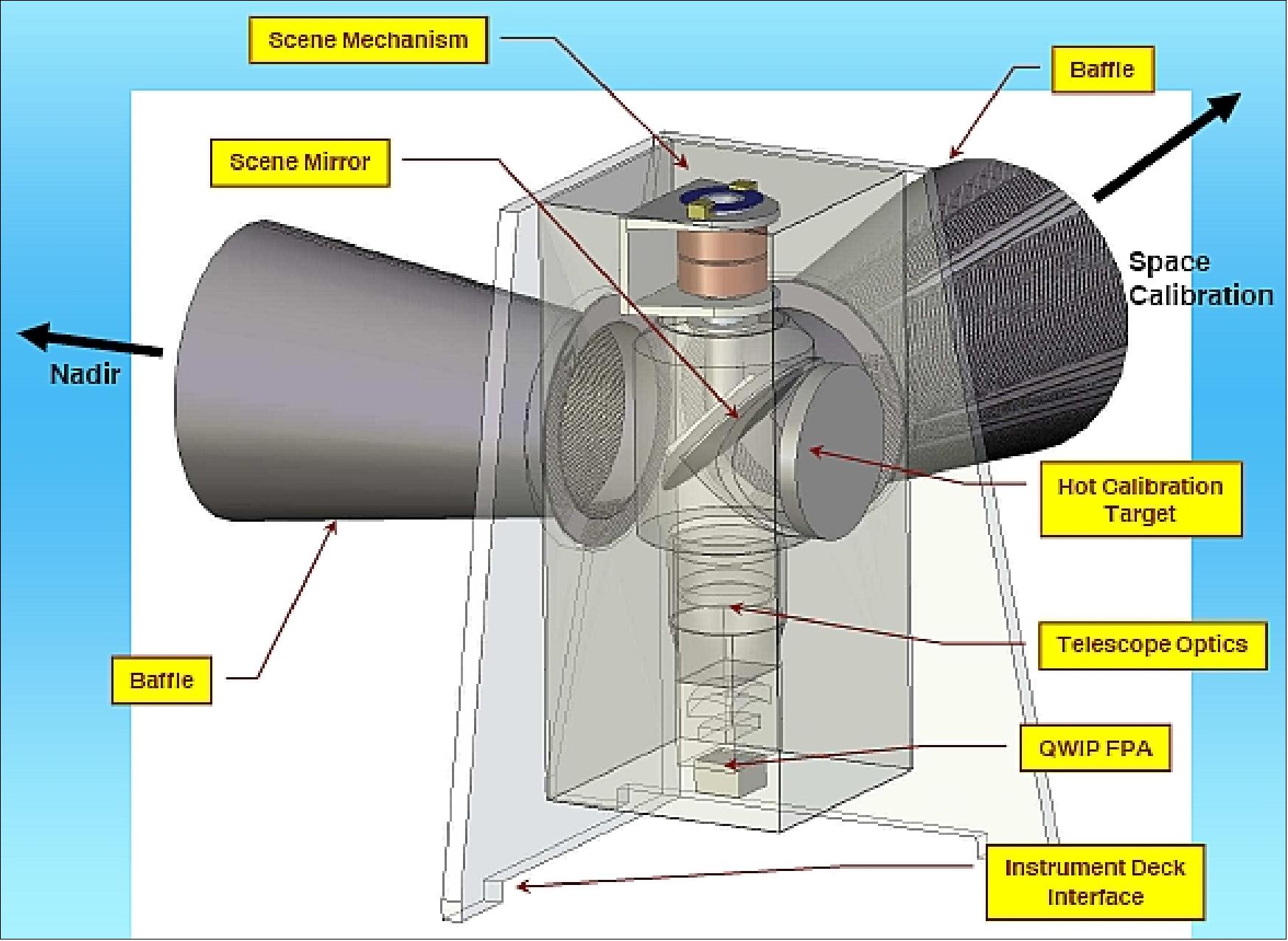
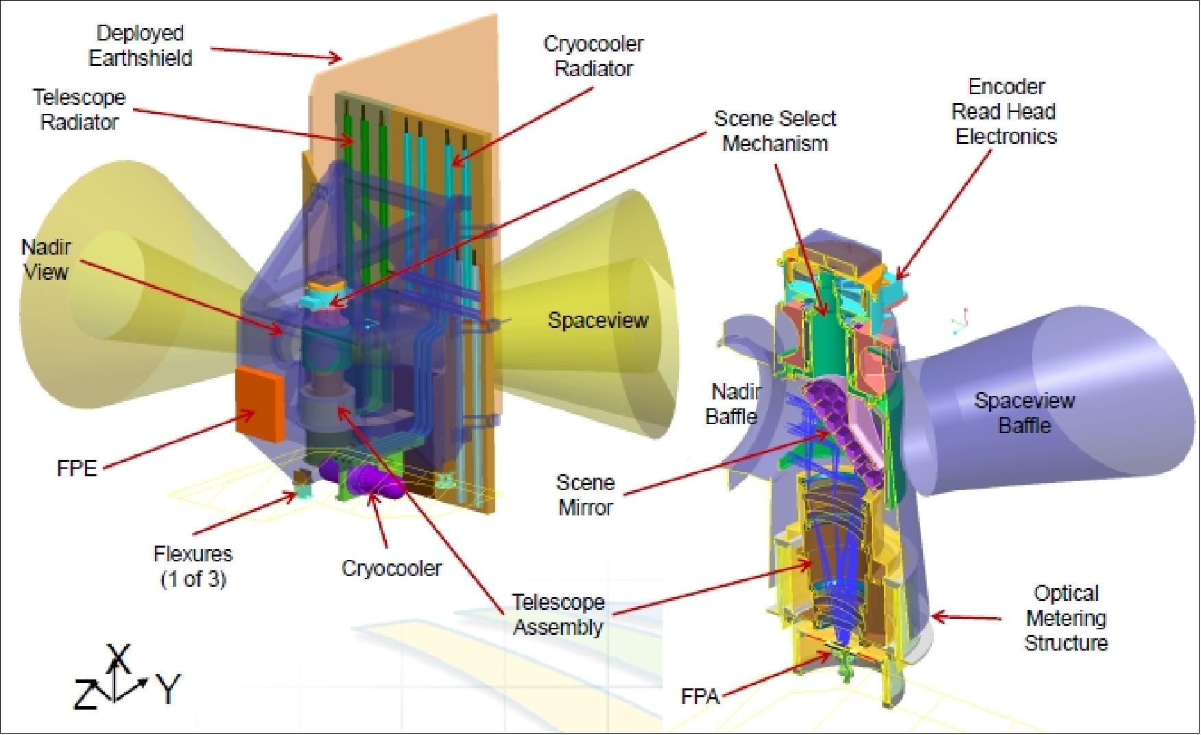
Legend to Figure 100: Model of the TIRS instrument showing the major components of the TIRS sensor. The scene select mechanism rotates the field of regard from the Earth view to either the space view or to the on-board calibrator. The right side provides some detail of optical system showing the 4-element lens, a cut-away view of the SM and the thermal strap connecting the FPA to the cryocooler cold tip. The MEB (Main Electronics Box) and the CCE (Cyrocooler and its associated Control Electronics), not shown, are mounted to the spacecraft.
TIRS Instrument Calibration
Consistent with previous Landsat missions, LDCM TIRS will be fully calibrated prior to launch. Calibration measurements will be made at GSFC and will be done at the component, subsystem and instrument level. NIST-traceable instrument level calibration will be done using an in-chamber calibration system. 103) 104)
Among other uses, TIRS data will be used to measure evapotranspiration (evaporation from soil and transpiration from plants); to map urban heat fluxes, to monitor lake thermal plumes from power plants; to identify mosquito breeding areas and vector-borne illness potential; and to provide cloud measurements. The evapotranspiration data may be used to estimate consumptive water use on a field-by-field basis.
TIRS instrument calibration makes use of the following elements:
• Precision scene select mirror to select between calibration sources and nadir view
• Two full aperture calibration sources
- Onboard variable temperature blackbody
- Space view
- Calibration every 34 minutes
• NIST Traceable radiometric calibration
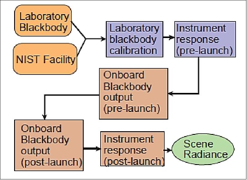
TIRS calibration system:
• A 41 cm diameter source is covering full field and aperture of TIRS (Flood Source)
• Target Source Module (GeoRadSource)
- Blackbody point source w/ filter & chopper
- All reflective, off-axis parabola collimator
- Motorized target and filter wheels
- A square steering mirror system (33 cm side length) is permitting coverage of the full aperture and field
• Cooled enclosure over entire system
• External monochromator (spectral source)
• Components are mounted to common base plate.
The TIRS radiometric response is determined via the prelaunch characterization relative to the laboratory blackbody. This approach provides the highest accuracy calibration. The calibration philosophy is then to evaluate (or validate) the calibration parameters once TIRS is on orbit. If the calibration of TIRS is demonstrated to change significantly while on orbit using measurements during the checkout period, then the on-board blackbody (OBB) will be used as the primary pathway to NIST traceability.
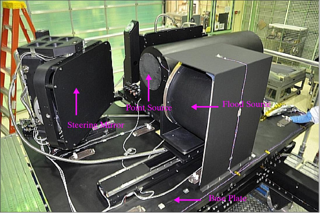
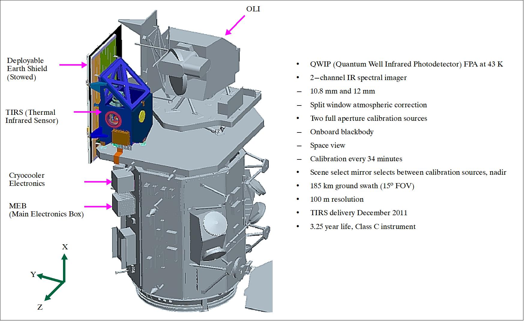
SSM (Scene Select Mechanism) of TIRS
The SSM for the TI RS instrument, developed at NASA/GSFC, is a single axis, direct drive mechanism which rotates a 207 mm scene mirror from the nadir science position to the 2 calibration positions twice per orbit. It provides pointing knowledge and stability to ~10 µradians. The SSM can be driven in either direction for unlimited rotations. The rotating mirror is dynamically balanced over the spin axis, and does not require launch locking. 105)
The design of the SSM is straightforward; it is a single axis rotational mechanism. The operational cadence was to hold the scene mirror stationary for ~40 minutes staring at nadir, rotate 120º to the space view aperture and stare for 30 seconds, rotate 120º to the internal blackbody and stare for 30 seconds and then rotate the mirror to the back to nadir. Then the entire process would start again. The mechanism would be operating all of the time, or have a 100% duty cycle. Since LDCM/TI RS was to be in a highly-inclined polar orbit, the general idea was to calibrate twice per orbit while over the poles.

Instrument mass, power | 15 kg, 6 W average |
Pointing knowledge, stability | ±9.7 µradians over 34 minutes, ±9.7 µradians over 2.5 seconds |
Duty cycle | 100% |
Thermal operational | 0 / +20ºC stable to ±1ºC |
Thermal survival range | -50 / +40ºC |
Lifetime | 3.25 years on orbit |
Redundancy | A/B side block redundancy |
Operational cadence | Stare nadir for 30-40 minutes |
Parameter | Landsat ETM+ | LDCM OLI | GMES/Sentinel-2 MSI | |||
Spectral bands | Band | µm | Band | µm | Band | µm |
|
| 1 (blue) | 0.43-0.45 | B1 (blue) | 0.43-0.45 | |
1 (blue) | 0.45–0.52 | 2 (blue) | 0.45–0.52 | B2 (blue) | 0.46–0.52 | |
2 (green) | 0.52–0.60 | 3 (green) | 0.52–0.60 | B3 (green) | 0.54–0.58 | |
3(red) | 0.63–0.69 | 4 (red) | 0.63–0.68 | B4 (red) | 0.65-0.68 | |
|
|
|
| B5 (red edge) | 0.70-0.71 | |
|
|
|
| B6 (red edge) | 0.73-0.75 | |
|
|
|
| B7 (red edge) | 0.77-0.79 | |
4 (NIR) | 0.76–0.90 |
|
| B8 (NIR) | 0.78-0.90 | |
|
| 5 (NIR) | 0.84-0.88 | B8a (NIR) | 0.86-0.88 | |
|
|
|
| B9 (water vapor) | 0.93-0.95 | |
|
| 9 (cirrus) | 1.36-1.39 | B10 (cirrus) | 1.37-1.39 | |
5 (SWIR1) | 1.55–1.75 | 6 (SWIR1) | 1.56-1.66 | B11 (SWIR1) | 1.57-1.66 | |
7 (SWIR2) | 2.08–2.35 | 7 (SWIR2) | 2.10-2.30 | B12 (SWRIR2) | 2.10-2.28 | |
|
| LDCM TIRS |
|
| ||
6 (TIR) | 10.4–12.5 | 10 (TIR1) | 10.3-11.3 |
|
| |
|
| 11 (TIR2) | 11.5-12.5 |
|
| |
GSD at nadir | 30 m VNIR | 30 m VNIR | 10 m (B2, B3, B4, B8) | |||
Quantization | 8 bit | 12 bit | 12 bit | |||
Onboard Calibration | Yes | Yes | Yes | |||
Resivit time | 16 days | 16 days | 5 days (2 satellites) | |||
Off-axis viewing | Up to 7.5º off nadir | Up to 7.5º off nadir | Up to 10.3º off nadir (w/o pointing) | |||
Orbit altitude | 705 km | 705 km | 786 km | |||
Swath width | 185 km | 185 km | 290 km | |||
Architecture | Cross-track scanner (Whiskbroom) | Pushbroom | Pushbroom | |||
Collection of Imagery Inboard LDCM
The co-aligned instruments are nominally nadir pointed and sweep the ground track land surface in contiguous image data collections, also known as image intervals. Each image interval may contain from a few WRS-2 scenes for an island or coastal area up to 77 contiguous WRS-2 scenes for an extended area of interest. For each image interval, the observatory executes a pre-defined imaging and ancillary data collection sequence as shown in Figure 105. 107)
Prior to the image interval, the spacecraft configures the onboard systems for the mission data collection session. A specific number of intervals are pre-defined on the ground based upon the number of WRS-2 scenes scheduled for collection, and allocated in the SSR (Solid State Recorder). Each instrument will transmit focal plane sensor data and instrument ancillary data (voltages, temperatures, etc.), which the spacecraft will interleave with the spacecraft ancillary data (attitude, ephemeris, etc), and record to files in the SSR.
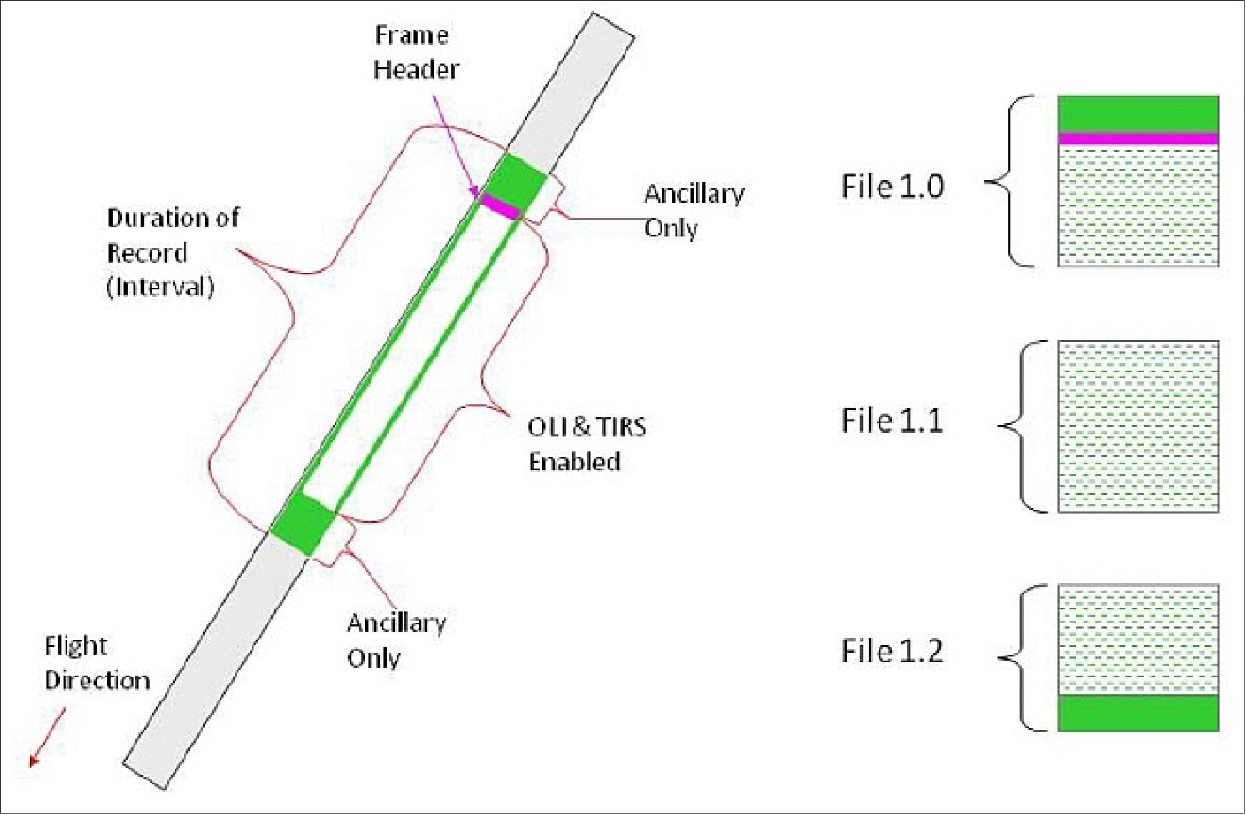
If the observatory is over an IC (International Cooperatoror) or LGN (Landsat Ground Network) station, it will simultaneously transmit data in real time to the ground. In addition, each instrument performs routine on-board calibrations (blackbody, lamps, etc) before and after each image interval, and during less frequent occasions utilizing the sun and moon as external calibration sources. A representation of the global image collection and calibration opportunities within the WRS-2 grid is shown in the 16-day repeating DRC-16 (Design Reference Case-16) in Figure 106.
The DRC-16 was developed to aid the mission architects in identification of all image and calibration activities and to verify that all are consistent with spacecraft power and mission data management capabilities. Instrument solar, lunar, and internal calibrations are required by ground system processing systems for image reconstruction, and to produce finished and distributable image products.
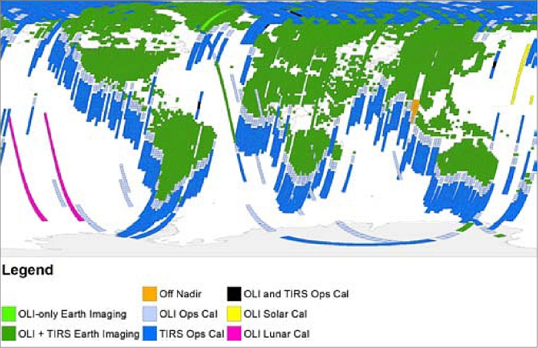
End to end mission data flow is represented in Figure107 . Mission data originates as instrument sensor (or “image”) data, and are collected and processed by the instrument electronics. The instrument electronics transmits the image data to the spacecraft PIE (Payload Interface Electronics) over a HSSDB (High Speed Serial Data Bus), using a serializer-deserializer integrated circuit pair. OLI image data are compressed using the USES (Universal Source Encoder for Space) ASIC (Application-Specific Integrated Circuit), which implements the Rice algorithm for lossless compression. - TIRS data are not compressed due to the low data rate. Instrument image data are interleaved with spacecraft ancillary data to create a file, which is stored and/or provided to the transmitter for downlink.
Ancillary data are collected at rates up to 50 Hz, and is comprised of GPS (Global Positioning System) data, IMU (Inertial Measurement Unit) data, star tracker data, and select instrument engineering information required by ground system algorithms for image product generation. The ancillary data are multiplexed within the mission data files every second.
Mission data files are intentionally fixed in size at 1GB. A system architecture trade study was performed early in mission definition to establish the optimum file size given the implementation of Class 1 CCSDS (Consultative Committee for Space Data Systems) CFDP (File Delivery Protocol), and a required link BER (Bit Error Rate) of < 10-12. Utilizing the 440 Mbit/s available downlink capacity, each downlinked mission data file requires 22 seconds of continuous transmission for a completed delivery to the ground system. The low BER requirement on the communication link provides the confidence that only one file over several days would require retransmission, well within the available contact time with the ground stations.
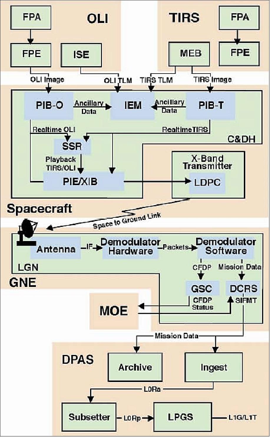
Simultaneous real-time and playback mission data files are transmitted to the ground through virtual channels within a single physical channel. Five data streams on the transmitter interface board may be multiplexed on to the link via an arbiter, which interleaves the data streams according to a pre-established priority scheme. The data streams priorities are:
1) Real-time for the OLI instrument
2) Real-time for the TIRS instrument
3) SSR playback channel 1
4) SSR playback channel 2
5) A virtual channel for fill frames in case no image data are available for downlink.
The five virtual channels are arbitrated in priority order on a frame-by-frame basis. The OLI instrument has the highest priority followed by the TIRS instrument and, since the combined mission data rates are less than the total downlink bandwidth available, there is always residual bandwidth available for mission data playback. This enables maximum utilization of the downlink bandwidth. SSR playback 1 has priority over SSR playback 2. SSR playback 2 is controlled by an autonomous on-board spacecraft flight software task that queues files for playback by a predefined algorithm (i.e. oldest to newest priority files first, oldest to newest non-priority files next).
SSR playback 1 is specifically for ground system intervention, as required to supersede the onboard autonomous SSR playback 1, to downlink files which are a higher priority than originally categorized. SSR playback 2 will resume automatically upon the completion of SSR playback 1 ground commands, and there is no need to stop and restart the autonomous SSR playback 2 queue. As a frame finishes transmission, the priority arbiter selects the highest priority channel that has a frame buffer ready for transmission for the next frame.
To ensure the bandwidth of the space to ground data link is at least twice the bandwidth of the real-time mission data, the spacecraft compresses OLI image data in near real time using CCSDS compression. During early hardware development, using simulated data derived from the ALI (Advanced Land Imager) sensor aboard the EO-1 (Earth Observing-1) satellite (the precursor to the OLI instrument), data sets were constructed and flowed through the compression chip and achieved a nominal 1.55:1 compression. As compression varies on the OLI real-time virtual channel, the playback capacity also varies to use the bandwidth that is available.
The multiplexed virtual channels of mission data are provided to the RF X-band subsystem, where the transmitter adds CCSDS layers and LDPC (Low Parity Density Check) 7/8-rate forward error correction to the 384 Mbit/s data stream, resulting in a 440 Mbit/s stream from the X-band subsystem. The X-band stream is modulated, amplified and down-linked from the spacecraft antenna to the ground station antenna/receivers.
The ground station antenna system receives the 8200.5 MHz OQPSK (Offset-keyed Quadrature Phase Shift Keying) X-band signal from the observatory and forwards the down converted 1.2 GHz or 720 MHz intermediate frequency (IF) signal to a programmable telemetry receiver. The IF signals are routed through a matrix switch, providing signal distribution or routing to redundant equipment as needed.
Within the programmable telemetry receiver, the IF signal from the switching matrix is subject to low-pass filtering to prevent subsequent aliasing followed by an AGC (Automatic Gain Control) action. The AGC action is the last analog handling of the signal prior to the digitizer. The entire ground processing that remains is accomplished in the digital domain. The signal is immediately digitally demodulated within a specially designed modified Costas loop and the resultant baseband signal, now a softbit stream, is sent to the bit synchronizer. The bit stream has ambiguity resolved and is then frame synchronized. The frame synchronizer parses the data stream into equal length frames; queuing on a predefined frame synchronization pattern. The data are de-randomized using the conventional CCSDS algorithm and then stripped of parity and bit-corrected by the LDPC 7/8-rate FEC (Forward Error Correction) decoder.
The frame synchronization processor routes the framealigned data stream to the VCDU (Virtual Channel Data Unit) processor. The VCDU processor identifies the unique virtual channels within the frames and outputs these VCDU into individual data streams for packet processing.
The mission data stream from the VCDU processor is processed through the CCSDS packet processor to separate APID (Application Process Identifiers). The packet processor outputs the resulting mission stream to the CFDP processor.
Landsat-8 / LDCM Ground System
The LDCM ground system includes all of the ground-based assets needed to operate the LDCM observatory. The primary components of the ground segment are : 108) 109) 110)
- MOE (Mission Operations Element)
- CAPE (Collection Activity Planning Element)
- GNE (Ground Network Element)
- DPAS (Data Processing and Archive System).
The USGS (United States Geological Survey) -and their associated support and development contractors - will:
- Develop the Ground System (comprised of the Flight Operations and Data Processing and Archive Segments), excluding procurement of the MOE
- Provide ground system functional area expertise across all mission segments
- Lead, fund, and manage the Landsat Science Team
- Acquire the FOT (Flight Operations Team) and produce the FOT products 111)
- Lead the LDCM mission operations, after the completion of the on-orbit checkout period
- Accept and execute all responsibilities associated with the transfer of the LDCM OLI (Operational Land Imager) instrument, TIRS (Thermal Infrared Sensor) instrument, spacecraft bus and Mission Operations Element contracts from NASA following on-orbit acceptance of the LDCM system including assuming contract management”
- Provide system engineering for the USGS-managed segments and elements.
The MOE is being provided by the Hammer Corporation. The MOE contract was awarded in September 2008. The MOE provides capability for command and control, mission planning and scheduling, long-term trending and analysis, and flight dynamics analysis. The overall activity planning for the mission is divided between the MOE and CAPE. The MOE hardware and software systems reside in the LDCM MOC (Mission Operations Center).
The CAPE develops a set of image collection and imaging sensor(s) calibration activities to be performed by the observatory. The CAPE schedules activities on a path-row scene basis. The MOE converts CAPE-generated path-row scenes to observatory activities, schedules these and any other detailed observatory activities, and generates commands necessary to collect the identified scenes and operate the observatory.
The GNE is comprised of two nodes located at Fairbanks, Alaska and Sioux Falls, SD. Each node in the GNE includes a ground station that will be capable of receiving LDCM X-band data. Additionally, each station provides complete S-band uplink and downlink capabilities. The GNE will route mission data and observatory housekeeping telemetry to the DPAS.
The DPAS includes those functions related to ingesting, archiving, calibration, processing, and distribution of LDCM data and data products. It also includes the portal to the user community. The ground system, other than the MOE, is developed by USGS largely through their support service contract. The DAPS will be located at the USGS EROS (Earth Resources Observation and Science) Center in Sioux Falls, SD.
Data access policy: All Landsat data are freely available over the Internet.
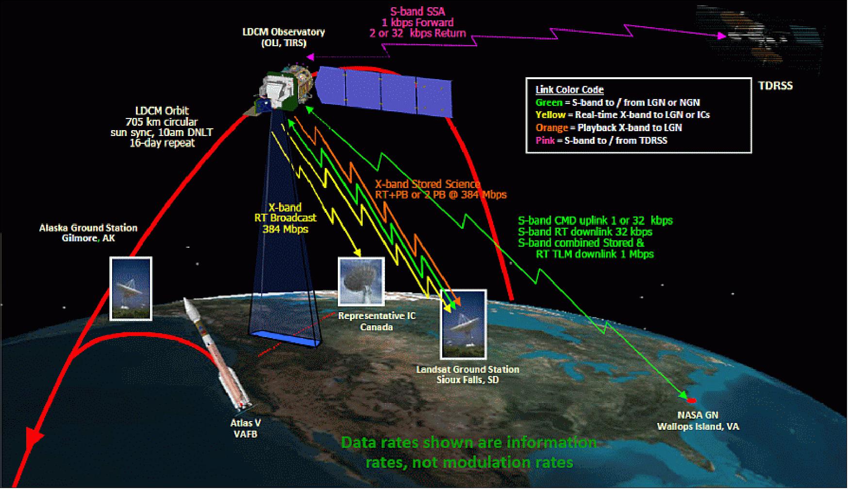
LGN (LDCM Ground Network) stations: The LGN is a collection of ground stations with state of the art electronics and sophisticated ground software, each providing similar mission services. The configuration of LGN uses the ground stations located at the EROS Center campus in Sioux Falls, South Dakota, the GLC (Gilmore Creek) ground station in Fairbanks, Alaska, and the SvalSat (Svalbard Satellite Station) ground station in Svalbard (Spitsbergen), Norway.
Each LGN ground station consists of a tracking antenna, S-band and X-band communication equipment, mission data storage and a file routing DCRS (Data Collection and Routing Subsystem). The LGN antenna receives X-band mission data files (autonomous playback or commanded) from the observatory, while simultaneously performing file management and subsequent image collection operations over S-band. The S-band and X-band systems of each LGN station interfaces with the MOE and DPAS in a closed loop fashion.
The USGS maintains agreements with several foreign governments referred to as the Landsat ICs (International Cooperators). The ICs are a special user community that has the ability to receive LDCM mission data from the observatory real-time X-band downlink stream. Real-time imaging sensor and ancillary data (including spacecraft and calibration data) required to process the science data are contained within the real-time stream downlink.
The ICs will be capable of receiving real-time X-band imaging sensor data downlinks and sending metadata to the DPAS. The ICs will submit imaging sensor data collection and downlink requests to the CAPE (via the DPAS user portal). ICs participate in a bilateral DV&E (Data Validation & Exchange) program with the DPAS. This program includes exchange of archive data upon request, and validation of IC processed level 1 data products by the USGS.
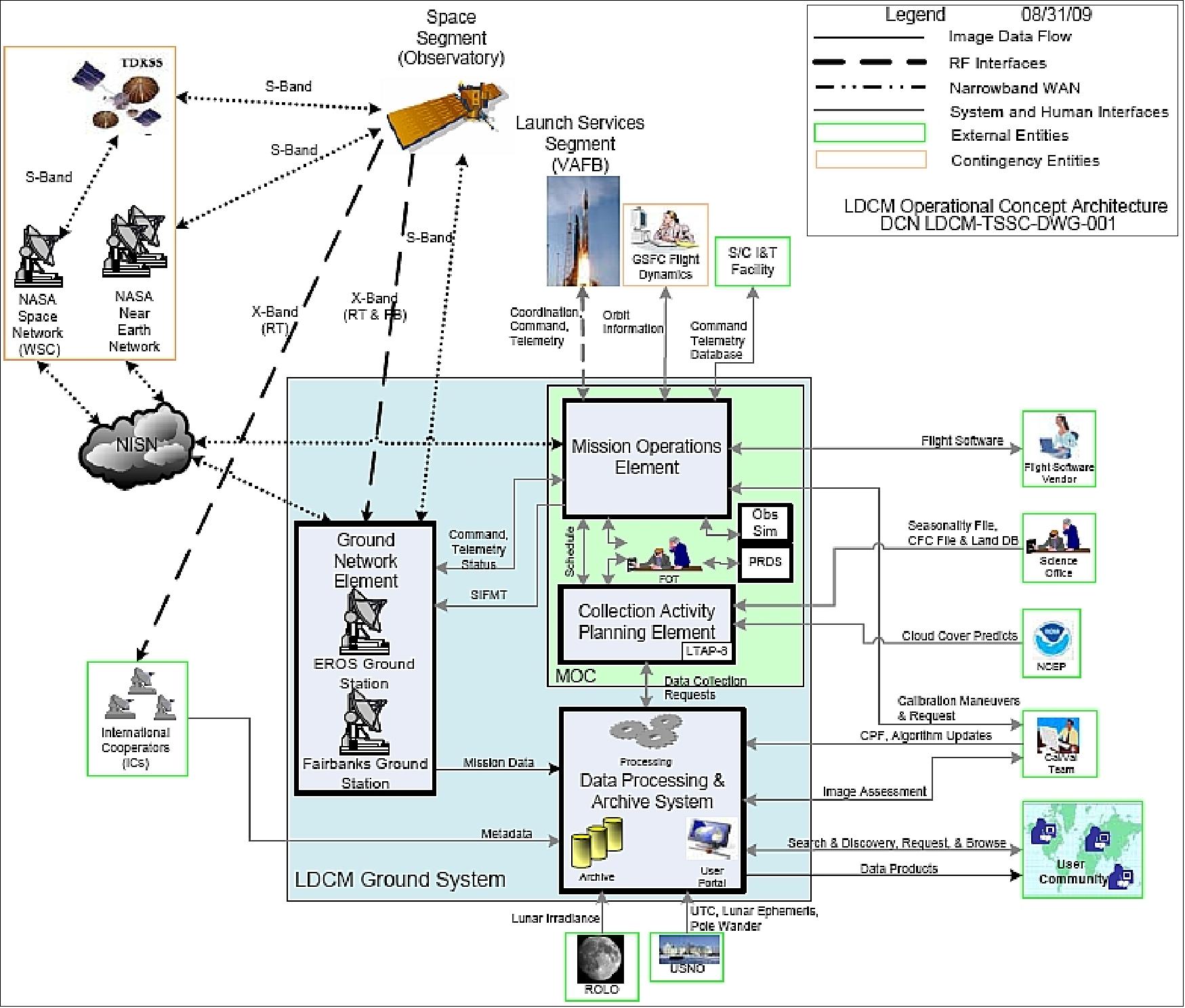
Item | Parameter | Total size |
System | Daily volume of 400 scenes | 390 GByte |
Spacecraft | C&DH data rate | 260.92 Mbit/s |
Space to ground communication | Downlink data rate | 384 Mbit/s data, 441 Msample/s symbol |
Ground station | Minutes per day (14 contacts) | 98 minutes |
Science archive | 5 year archive | ~ 400 TB |
IC (International Cooperator) Ground Stations of the Landsat Program
• In 41 years, 39 IC stations in 23 countries
• Most still collect and/or distribute Landsat products, reducing the load on U.S. Systems
• More than 215,000 products distributed in 2012
- Represents a nearly 10% off-loading of network bandwidth
- Enhanced regional exploitation of Landsat data
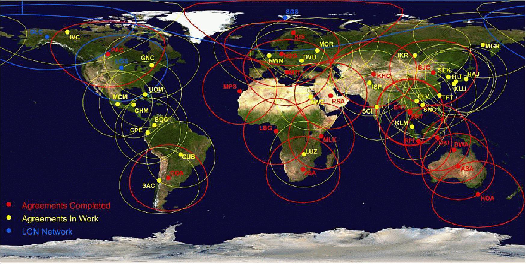
IAS (Image Assessment System)
Once the LDCM spacecraft is in orbit, the radiometric, geometric and spatial performance of OLI and TIRS sensors will be continually monitored, characterized and calibrated using the IAS (Ref. 93).
Background: The IAS was originally developed to monitor radiometric and geometric performance of the Landsat-7 ETM+ sensor and the quality of the image data in the Landsat-7 archive. The operational performance monitoring is achieved by processing a number of randomly selected Level 0R (raw reformatted) images to Level 1R (radiometrically corrected) and Level 1G (geometrically corrected) products. In that process, image statistics at different processing levels, calibration data, and telemetry data are extracted and stored in the IAS database for automatic and off-line assessment. The IAS also processes and analyzes the pre-selected geometric and radiometric calibration sites and special calibration acquisitions, e.g. solar diffuser or night data needed for radiometric calibration or noise and stability studies. The final and most important product of the IAS trending and processing is the CPF (Calibration Parameter File), the file that contains parameters needed for artifact corrections and radiometric and geometric processing of raw image data. To maintain the accuracy of the dynamic parameters, the CPF is updated at least once every three months.
The purpose of the LDCM IAS is to maintain accurate spectral, radiometric, spatial and geometric characterization and calibration of LDCM data products and sensors, ensuring compliance with the OLI and TIRS data quality requirements. The IAS will trend results of processing standard Earth images and nonstandard products, such as lunar, solar, dark Earth or stellar images, evaluate image statistics and calculate and store image characteristics for further analysis.
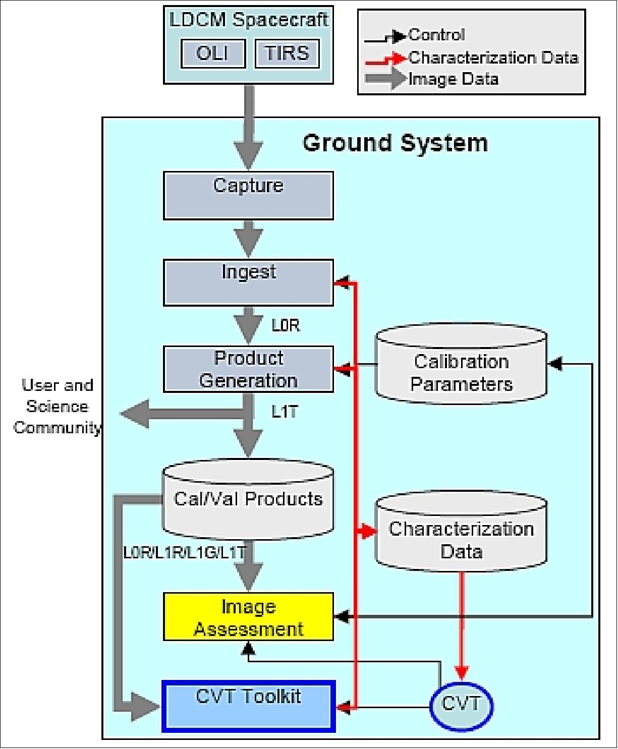
The IAS will automatically generate calibration parameters, which will be evaluated by the calibration analysts. In addition to standard operations within the IAS, the CVT (Calibration and Validation Team) will use a ‘toolkit’ module containing instrument vendor developed code and routines developed by the CVT, as a research and development environment for improvements of algorithm functionality and anomaly investigations.
Compared to the previous IAS versions, the LDCM IAS system will have to handle a significantly larger and more complex database that will include characterization data from all normally acquired images (~ 400 scenes per day, with special calibration acquisitions, e.g solar and lunar) processed through the product generation system. OLI’s pushbroom design (~ 75000 detectors), as opposed to an ETM+ whiskbroom design, requires characterization and calibration of about 550 times more detectors than in case of ETM+ (136 detectors) and represents a major challenge for the LDCM IAS. An additional challenge is that the LDCM IAS must handle data from two sensors, as the LDCM products will contain both the OLI and TIRS data.
For radiometric and geometric processing, see Ref. 93).
• Processing latency for real-time downlinks • Average latency is ~ 5 hours from acquisition to product availability • Closed loop between ground and space for data management • The system requirement calls for 85% data availability to the user community through EROS Portal within 48 hours. The actual performance for Landsat-8 averages within 5 hours. |
Landsat-8 Reprocessing
• All Landsat 8 data is being reprocessed to make corrections based on first year data analysis.
• Corrections to both OLI (Operational Land Imager) and the TIRS (Thermal Infrared Sensor) data are being made including:
- all calibration parameter file updates since launch
- improved OLI reflectance conversion coefficients for the cirrus band
- improved OLI radiance conversion coefficients for all bands
- refined OLI detector linearization to decrease striping
- a radiometric offset correction for both TIRS bands
- a slight improvement to the geolocation of the TIRS data
• Approximately 90% of reprocessing is completed with estimated completion by March 30, 2014.
Landsat: Continuing the Legacy
April 1, 2021: Five decades ago, NASA and the U.S. Geological Society launched a satellite to monitor Earth’s landmasses. The Apollo era had given us our first look at Earth from space and inspired scientists to regularly collect images of our planet. The first Landsat — originally known as the Earth Resources Technology Satellite (ERTS) — rocketed into space in 1972. Today we are preparing to launch the ninth satellite in the series. 114)
Each Landsat has improved our view of Earth, while providing a continuous record of how our home has evolved. We decided to examine the legacy of the Landsat program in a four-part series of videos narrated by actor Marc Evan Jackson (who played a Landsat scientist in the movie Kong: Skull Island). The series moves from the birth of the program to preparations for launching Landsat 9 and even into the future of these satellites.
The soon-to-be-launched, Landsat-9 is the intellectual and technical successor to eight generations of Landsat missions. Episode 1 answers the “why?” questions. Why did space exploration between 1962 and 1972 lead to such a mission? Why did the leadership of several U.S. government agencies commit to it? Why did scientists come to see satellites as important to advancing earth science? In this episode, we are introduced to William Pecora and Stewart Udall, two men who propelled the project forward, as well as Virginia Norwood, who breathed life into new technology.
The early Landsat satellites carried a sensor that could “see” visible light, plus a little bit of near-infrared light. Newer Landsats, including the coming Landsat 9 mission, have two sensors: the Operational Land Imager (OLI) and the Thermal Infrared Sensor (TIRS). Together they observe in visible, near-infrared, shortwave-infrared, and thermal infrared wavelengths. By comparing observations of different wavelengths, scientists can identify algal blooms, storm damage, fire burn scars, the health of plants, and more.
Episode 2 takes us inside the spacecraft, showing how Landsat instruments collect carefully calibrated data. We are introduced to Matt Bromley, who studies water usage in the western United States, as well as Phil Dabney and Melody Djam, who have worked on designing and building Landsat-9. Together, they are making sure that Landsat continues to deliver data to help manage Earth’s precious resources.
The Landsat legacy includes five decades of observations, one of the longest continuous Earth data records in existence. The length of that record is crucial for studying change over time, from the growth of cities to the extension of irrigation in the desert, from insect damage to forests to plant regrowth after a volcanic eruption. Since 2008, that data has been free to the public. Anyone can download and use Landsat imagery for everything from scientific papers to crop maps to beautiful art.
Episode 3 explores the efforts of USGS to downlink and archive five decades of Landsat data. We introduce Mike O’Brien, who is on the receiving end of daily satellite downloads, as well as Kristi Kline, who works to make Landsat data available to users. Jeff Masek, the Landsat 9 project scientist at NASA, describes how free access to data has revolutionized what we are learning about our home planet.
For the past 50 years, Landsat satellites have shown us Earth in unprecedented ways, but they haven’t operated in isolation. Landsat works in conjunction with other satellites from NASA, NOAA, and the European Space Agency, as well as private companies. It takes a combination of datasets to get a full picture of what’s happening on the surface of Earth.
In Episode 4, we are introduced to Danielle Rappaport, who combines audio recordings with Landsat data to measure biodiversity in rainforests. Jeff Masek also describes using Landsat and other data to understand depleted groundwater.
References
1) Bill Ochs, “Status of the Landsat Data Continuity Mission,” Landsat Science Team Meeting, Boise, Idaho, June 15-17, 2010, URL: http://landsat.usgs.gov/documents/June_2010_Ochs%20-%20NASA%20LDCM%20Project%20Status.pdf
2) Brian L. Markham, Philip W. Dabney, James C. Storey, Ron Morfitt, Edward J. Knight, Geir Kvaran, Kenton Lee, “Landsat Data Continuity Mission Calibration and Validation,” Proceedings of the Pecora 17 Memorial Remote Sensing Symposium, Denver, CO, USA, Nov. 18-20, 2008
3) Brian Markham, “Landsat Data Continuity Mission: Overview and Status,” 10th Annual JACIE ( Joint Agency Commercial Imagery Evaluation) Workshop, March 29-31, 2011, Boulder CO, USA, URL: http://calval.cr.usgs.gov/JACIE_files/JACIE11/Presentations/TuePM/310_Markham_JACIE_11.080.pdf
4) J. R. Irons, J. G. Masek, “Requirements for a Landsat Data Continuity Mission,” PE&RS, Vol. 72, No 10, Oct. 2006, pp. 1102-1108
5) “Landsat Data Continuity Mission,” NASA/GSFC, http://landsat.gsfc.nasa.gov/about/ldcm.html
7) J. D. McCuistion, C. D. Wende, J. R. Irons, “Landsat Data Continuity Mission: Creating a Unique Government-Industry Partnership for Global Research,” Proceedings of IGARSS 2003, Toulouse, France, July 21-25, 2003
8) J. R. Irons, N. J. Speciale, et al., “Data Specifications for the Landsat Data Continuity Mission,” Proceedings of IGARSS 2003, Toulouse, France, July 21-25, 2003
9) Landsat Data Continuity Mission (LDCM) Implementation Phase - Data Specification,” Jan. 6, 2003, URL: http://prod.nais.nasa.gov/eps/eps_data/102577-SOL-001-005.pdf
10) James Verdin, “The requirement for high quality data and information for Science,” 10th Annual JACIE ( Joint Agency Commercial Imagery Evaluation) Workshop, March 29-31, 2011, Boulder CO, USA, URL: http://calval.cr.usgs.gov/JACIE_files/JACIE11/Presentations/TueAM/1055_Verdin_JACIE2011.pdf
11) “Landsat Data Continuity Mission,” USGS, URL: http://pubs.usgs.gov/fs/2007/3093/pdf/fs20073093.pdf
12) J. Irons, “New Landsat Data Continuity Mission (LDCM) Memorandum from OSTP,” The Earth Observer, NASA/GSFC, Vol. 18, Issue 1, January-February 2006, pp. 4-5
13) “A Landsat Timeline,” NASA/GSFC, URL: http://landsat.gsfc.nasa.gov/?p=3166
14) “NASA, USGS Begin Work on Landsat 9 to Continue Land Imaging Legacy,” NASA, April 16, 2015, URL: http://www.nasa.gov/press/2015/april/nasa-usgs-begin-work-on-landsat-9-to-continue-land-imaging-legacy
15) Cynthia M. O'Carroll, ”NASA Awards Letter Contract for Landsat 9 Imager-2,” NASA, Dec. 31, 2015, URL: http://www.nasa.gov/press-release/goddard/nasa-awards-letter-contract-for-landsat-9-imager-2
16) “NASA selects contractor for Landsat Data Continuity Mission spacecraft,” April 22, 2008, URL: http://www.nasa.gov/home/hqnews/2008/apr/HQ_C08021_Landsat_Data.html
17) B. Berger, “Price the Deciding Factor in General Dynamics' LDCM Win,” Space News, May 5, 2008, p. 6
18) Bill Anselm, “LDCM Spacecraft Status,” June 23, 2009, URL: http://landsat.usgs.gov/documents/9_Anselm_Spacecraft_Report.ppt
19) Mike Wulder, Landsat Science Team, “Landsat Data Continuity Mission and Beyond,” 4th Global Vegetation Workshop, Missoula, MT, USA, June 16-19, 2009
20) http://www.orbital.com/SatellitesSpace/ScienceTechnology/LDCM/
21) James R. Irons, John L. Dwyer, “An overview of the Landsat Data Continuity Mission (LDCM),” Proceedings of the SPIE, Volume 7695, 2010, pp. 769508-769508-7, 'Algorithms and Technologies for Multispectral, Hyperspectral, and Ultraspectral Imagery XVI,' edited by Sylvia S. Shen, Paul E. Lewis, Paul, April 5-9, 2010, Orlando, FLA, USA,
22) Brian Markham, James Irons, Philip Dabney, “Landsat Data Continuity Mission,” Proceedings of IGARSS (International Geoscience and Remote Sensing Symposium), Vancouver, Canada, July 24-29, 2011
23) Kate Ramsayer, “Landsat Looks to the Moon,” NASA, July 11, 2014, URL: http://www.nasa.gov/content/goddard/landsat-looks-to-the-moon/#.U8SqX0C4Ri0
24) USGS, March 2, 2012, URL: http://landsat.usgs.gov/Landsat_Picture_Gallery.php
25) Steve Cole, George Diller, Rani Gran, “NASA Launches New Earth Observation Satellite to Continue 40-Year Legacy ,” NASA News Release 13-040, Feb. 11, 2013, URL: http://www.nasa.gov/home/hqnews/2013/feb/HQ_13-040_LDCM_Launches.html
26) NASA Selects Launch Services Provider for Earth Imagery Satellite,” Oct. 3, 2007, URL: http://landsat.gsfc.nasa.gov/news/news-archive/news_0104.html
27) Laurie M Mann, Susan M. Good, Ann M. Nicholson, Mark A. Woodard, “Landsat Data Continuity Mission (LDCM) Safe Operations Ascent Design,” Proceedings of SpaceOps 2012, The 12th International Conference on Space Operations, Stockholm, Sweden, June 11-15, 2012
28) ”Anatomy of Landsat 8, USGS satellite,” USGS, NASA, 13 June 2017, URL: https://www.youtube.com/watch?v=XiaXDomrooE&feature=youtu.be
29) ”Landsat Data Continuity Mission Overview,” NASA, 22 May 2013, URL: https://www.youtube.com/watch?v=mqVKR9OnqqA
30) ”Lake Mead Keeps Dropping,” NASA Earth Observatory, Image of the Day for22 July 2022, URL: https://earthobservatory.nasa.gov/images/150111/lake-mead-keeps-dropping
31) ”Blooming Lake Okeechobee,” NASA Earth Observatory, Image of the Day for 16 July 2022, URL: https://earthobservatory.nasa.gov/images/150093/blooming-lake-okeechobee
32) ”São Miguel, Azores,” NASA Earth Observatory, Image of the Day for 7 July 2022, URL: https://earthobservatory.nasa.gov/images/150034/sao-miguel-azores
33) ”Measuring War’s Effect on a Global Breadbasket,” NASA Earth Observatory, Image of the Day for 1 July 2022, URL: https://earthobservatory.nasa.gov/images/150025/measuring-wars-effect-on-a-global-breadbasket
34) ”Building Abuja,” NASA Earth Observatory, Image of the Day for 29 June 2022, URL: https://earthobservatory.nasa.gov/images/149937/building-abuja
35) ”Terceira Island, Azores,” NASA Earth Observatory, Image of the Day for 22 June 2022, URL: https://earthobservatory.nasa.gov/images/149982/terceira-island-azores
36) ”Freedom’s Fortress,” NASA Earth Observatory, Image of the Day for 19 June 2022, URL: https://earthobservatory.nasa.gov/images/149993/freedoms-fortress
37) ”Fire and Ice in Kamchatka,” NASA Earth Observatory, Image of the Day for 11 June 2022, URL: https://earthobservatory.nasa.gov/images/149966/fire-and-ice-in-kamchatka
38) ”A River Routed Under the Mountains,” NASA Earth Observatory, Image of the Day for 9 June 2022, URL: https://earthobservatory.nasa.gov/images/149941/a-river-routed-under-the-mountains
39) ”West Virginia’s Dark, Starry Parks,” NASA Earth Observatory, Image of the Day for 6 June 2022, URL: https://earthobservatory.nasa.gov/images/149904/west-virginias-dark-starry-parks
40) ”Melting Glacier Exposes Ichthyosaur Fossils,” NASA Earth Observatory, Image of the Day for 3 June 2022, URL: https://earthobservatory.nasa.gov/images/149894/melting-glacier-exposes-ichthyosaur-fossils
41) ”The Changing Seas of the Florida Keys,” NASA Earth Observatory, Image of the Day for 31 May 2022, URL: https://earthobservatory.nasa.gov/images/149886/the-changing-seas-of-the-florida-keys
42) ”Manam Volcano, Papua New Guinea,” NASA Earth Observatory, Image of the Day for 30 May 2022, URL: https://earthobservatory.nasa.gov/images/149883/manam-volcano-papua-new-guinea?src=eoa-iotd
43) ”The Black Fire Blows Up in New Mexico,” NASA Earth Observatory, Image of the Day for 24 May 2022, URL: https://earthobservatory.nasa.gov/images/149868/the-black-fire-blows-up-in-new-mexico
44) ”Maui’s Iconic Waves,” NASA Earth Observatory, Image of the Day for 16 May 2022, URL: https://earthobservatory.nasa.gov/images/149818/mauis-iconic-waves
45) ”The Emerald Isles of Ha Long Bay,” NASA Earth Observatory, Image of the Day for 7 May 2022, URL: https://earthobservatory.nasa.gov/images/149803/the-emerald-isles-of-ha-long-bay
46) ”Measuring Methane in the Everglades,” NASA Earth Observatory, Image of the Day for 5 May 2022, URL: https://earthobservatory.nasa.gov/images/149788/measuring-methane-in-the-everglades
47) ”Navigating the Geiyo Islands,” NASA Earth Observatory, Image of the Day for 30 April 2022, URL: https://earthobservatory.nasa.gov/images/149763/navigating-the-geiyo-islands
48) ”Ice Lost, Island Found?,” NASA Earth Observatory, Image of the Day for 27 April 2022, URL: https://earthobservatory.nasa.gov/images/149755/ice-lost-island-found
49) ”A Salty Sanctuary in Baja California Sur,” NASA Earth Observatory, Image of the Day for 25 April 2022, URL: https://earthobservatory.nasa.gov/images/149735/a-salty-sanctuary-in-baja-california-sur
50) ”The Great Barrier Reef Through Time,” NASA Earth Observatory, Image of the Day for 16 April 2022, URL: https://earthobservatory.nasa.gov/images/149724/the-great-barrier-reef-through-time
51) Jody M. Webster, Juan Carlos Braga, Marc Humblet, Donald C. Potts, Yasufumi Iryu, Yusuke Yokoyama, Kazuhiko Fujita, Raphael Bourillot, Tezer M. Esat, Stewart Fallon, William G. Thompson, Alexander L. Thomas, Hironobu Kan, Helen V. McGregor, Gustavo Hinestrosa, Stephen P. Obrochta & Bryan C. Lougheed,” Response of the Great Barrier Reef to sea-level and environmental changes over the past 30,000 years,” Nature Geoscience, Volume 11, pp: 426-432, Published: 28 May 2018, https://doi.org/10.1038/s41561-018-0127-3
52) J. M. Pandolfi, Russell Kelley, ” The Great Barrier Reef in Time and Space: Geology and Palaeobiology,” January 2011, URL: https://tinyurl.com/yaby2dvh
53) ”A Renewable Future for Fukushima,” NASA Earth Observatory, Image of the Day for 14 April 2022, URL: https://earthobservatory.nasa.gov/images/149711/a-renewable-future-for-fukushima
54) ”Great Barrier Reef Mass Bleaching Event,” NASA Earth Observatory, Image of the Day for 7 April 2022, URL: https://earthobservatory.nasa.gov/images/149666/great-barrier-reef-mass-bleaching-event
55) ”World’s Longest Wave?,” NASA Earth Observatory, Image of the Day for 1 April 2022, URL: https://earthobservatory.nasa.gov/images/149605/worlds-longest-wave
56) ”Not So Green Houses,” NASA Earth Observatory, 13 March 2022, URL: https://earthobservatory.nasa.gov/images/149573/not-so-green-houses
57) ”Sri Lanka’s Granite Fortress,” NASA Earth Observatory, Image of the Day for 5 March 2022, URL: https://earthobservatory.nasa.gov/images/149543/sri-lankas-granite-fortress
58) ”Young Impact Crater Uncovered in Yilan,” NASA Earth Observatory, Image of the Day for 27 February 2022, URL: https://earthobservatory.nasa.gov/images/149515/young-impact-crater-uncovered-in-yilan
59) ”Soaking Up Sun in the Thar Desert,” NASA Earth Observatory, Image of the Day for 19 February 2022, URL: https://earthobservatory.nasa.gov/images/149442/soaking-up-sun-in-the-thar-desert
60) ”Iberian Peninsula Drought,” NASA Earth Observatory, Image of the Day for 16 February 2022, URL: https://earthobservatory.nasa.gov/images/149469/iberian-peninsula-drought
61) ”Chilean Volcano Low on Snow,” NASA Earth Observatory, Image of the Day for 15 February 2022, URL: https://earthobservatory.nasa.gov/images/149463/chilean-volcano-low-on-snow
62) ”A Lake in Winter,” NASA Earth Observatory, Image of the Day for 9 February 2022, URL: https://earthobservatory.nasa.gov/images/149438/a-lake-in-winter
63) ”A Satellite View of Olympic Terrain,” NASA Earth Observatory, Image of the Day for7 February 2022, URL: https://earthobservatory.nasa.gov/images/149430/a-satellite-view-of-olympic-terrain
64) ”Island Nation Hit Hard by Eruption,” NASA Earth Observatory, Image of the Day for 31 January 2022, URL: https://earthobservatory.nasa.gov/images/149391/island-nation-hit-hard-by-eruption
65) ”Guishan Island,” NASA Earth Observatory, Image of the Day for 22 January 2022, URL: https://earthobservatory.nasa.gov/images/149363/guishan-island
66) ”Ice Age Canadian Lakes,” NASA Earth Observatory, Image of the Day for 21 January 2022, URL: https://earthobservatory.nasa.gov/images/149352/ice-age-canadian-lakes
67) ”Everest-Area Plant Life Spreads,” NASA Earth Observatory, Image of the Day for12 January 2022, URL: https://earthobservatory.nasa.gov/images/149312/everest-area-plant-life-spreads
68) ”A View of Vesuvius,” NASA Earth Observatory, Image of the Day for 10 January 2022, URL: https://earthobservatory.nasa.gov/images/149298/a-view-of-vesuvius
69) ”A Different Shade of Ice,” NASA Earth Observatory, Image of the Day for 4 January 2022, URL: https://earthobservatory.nasa.gov/images/149283/a-different-shade-of-ice
70) Steve Cole, Kate Ramsayer, Jon Campbell, “Landsat 8 Satellite Begins Watch,” NASA Release 13-160, May 30, 2013, URL: http://www.nasa.gov/home/hqnews/2013/may/HQ_13-160_Landsat_8_Begins.html
71) Kate Ramsayer, “NASA's Landsat Satellite Looks for a Cloud-Free View,” NASA, May 22, 2013, URL: http://www.nasa.gov/mission_pages/landsat/news/cloud-free-aral.html
72) Jon Campbell, “Landsat Images Provide the Gold Standard for New Earth Applications,” USGS News rooms, May 9, 2013, URL: http://www.usgs.gov/newsroom/article.asp?ID=3586&from=rss_home
73) Rebecca Moore, “A picture of Earth through time,” Google Official Blog, May 9, 2013, URL: http://googleblog.blogspot.de/
74) Steve Cole, “New Public Application of Landsat Images Released,” NASA, May 9, 2013, URL: http://www.nasa.gov/mission_pages/landsat/news/google-engine.html
75) “LDCM Mission Updates,” NASA, URL: http://www.nasa.gov/mission_pages/landsat/main/mission-updates.html
76) “Landsat Thermal Sensor Lights Up from Volcano's Heat,” NASA, May 6, 2013, URL: http://www.nasa.gov/mission_pages/landsat/news/indonesia-volcano.html
77) “Landsat Data Continuity Mission,” NASA, News and Features, URL: http://www.nasa.gov/mission_pages/landsat/news/index.html
78) “LDCM Status Update for May 2, 2013,” NASA, May 15, 2013, URL: http://www.nasa.gov/mission_pages/landsat/main/mission-updates.html
79) Matt Radcliff, Rob Simmon, Jesse Allen, Holli Riebeek, Paul Przyborski, “Come Fly With the Newest Landsat,” NASA Earth Observatory, URL: http://earthobservatory.nasa.gov/Features/LDCMLongSwath/?src=features-recent
80) Tom Holm, “Landsat: Building a Future on 40 Years of Success - April 14, 2013, 705 km Orbit,” 12th Annual JACIE (Joint Agency Commercial Imagery Evaluation) Workshop , St. Louis, MO, USA, April 16-18, 2013, URL: http://calval.cr.usgs.gov/wordpress/wp-content/uploads/JACIE-LDCM-Status-and-Overview-v4.pdf
81) “LDCM Underfly with Landsat 7,” USGS, March 29, 2013, URL: http://landsat.usgs.gov/LDCM_Underfly_with_Landsat_7.php
82) Steve Cole, Jon Campbell, “First Images Released From Newest Earth Observation Satellite,” NASA, USGS, March 21, 2013, URL: http://www.nasa.gov/home/hqnews/2013/mar/HQ_13-080_LDCM_Images.html
83) “A Closer Look at LDCM's First Scene,” NASA, March 21, 2013, URL: http://www.nasa.gov/mission_pages/landsat/news/first-images-feature.html
84) “LDCM Status Update for Feb. 21,” NASA, Feb. 21, 2013, URL: http://www.nasa.gov/mission_pages/landsat/main/index.html
85) “NASA Completes Critical Design Review Of One Landsat Instrument,” Space Daily, May 28, 2010, URL: http://www.spacedaily.com/reports/NASA_Completes_Critical_Design_Review_Of_One_Landsat_Instrument_999.html
86) Bryant Cramer, “USGS Perspectives on LDCM and Landsat,” Landsat Science Team Meeting,” Jan. 19-21, 2010, Mountain View, CA, USA, URL: http://landsat.usgs.gov/documents/Jan_2010_Cramer_01_19_10Landsat_Future_BriefingLSTtnv2.pdf
87) Tom Loveland, “Landsat and LDCM Status,” 2008 NASA Carbon Cycle & Ecosystems Joint Science Workshop, April 28-May 2, 2008, University of Maryland, Adelphi, MD, USA
88) James Storey, Michael Choate, Kenton Lee, “Geometric performance comparison between the OLI and ETM+,” Proceedings of the Pecora 17 Memorial Remote Sensing Symposium, Denver, Co, USA, Nov. 16-20, 2008
89) Jeanine Murphy-Morris, “Operational Land Imager ,” Landsat Science Team Meeting, Sioux Falls, SD, Jan. 8, 2008, URL: http://landsat.usgs.gov/documents/Murphy_Morris_Science_Team_OLI_chart.ppt
90) Edward J. Knight, “OLI Overview and Status,” Landsat Science Team Meeting, July 15, 2008, Reston, VA, URL: http://landsat.usgs.gov/documents/Knight_OLI.pdf
91) Bill Ochs, “Status of the Landsat Data Continuity Mission,” Landsat Science Team Meeting, July 15, 2008, Reston, VA, URL: http://landsat.usgs.gov/documents/Ochs_LDCM_Status.pdf
92) Edward J. Knight, Brent Canova, Eric Donley, Geir Kvaran, Kenton Lee, “The Operational Land Imager:Overview and Performance,” 10th Annual JACIE ( Joint Agency Commercial Imagery Evaluation) Workshop, March 29-31, 2011, Boulder CO, USA, URL: http://calval.cr.usgs.gov/JACIE_files/JACIE11/Presentations/TuePM/325_Knight_JACIE_11.070.pdf
93) Esad Micijevic, Ron Morfitt, “Operational Calibration and Validation of Landsat Data Continuity Mission (LDCM) Sensors using the Image Assembly System (IAS),” Proceedings of IGARSS (IEEE International Geoscience and Remote Sensing Symposium) 2010, Honolulu, HI, USA, July 25-30, 2010
94) Brian L. Markham, Philip W. Dabney, Edward J. Knight, Geir Kvaran, Julia A. Barsi, Jeanine E. Murphy-Morris, Jeffrey A. Pedelty, “The Landsat Data Continuity Mission Operational Land Imager (OLI) Radiometric Calibration,” Proceedings of IGARSS (IEEE International Geoscience and Remote Sensing Symposium) 2010, Honolulu, HI, USA, July 25-30, 2010, URL: http://ntrs.nasa.gov/archive/nasa/casi.ntrs.nasa.gov/20100026050_2010028396.pdf
95) Brian Markham, “LDCM On-Orbit Cal/Val Considerations,” Proceedings of the Landsat Science Team Meeting, Mesa, AZ, USA, March 1-3, 2011, URL: http://landsat.usgs.gov/documents/LDCM_Cal_Val_Considerations.pdf
96) “Ball Aerospace Completes CDR For Landsat's Operational Land Imager,” Nov. 26, 2008, Spacemart, URL: http://www.spacemart.com/reports/Ball_Aerospace_Completes_CDR_For_Landsat_Operational_Land_Imager_999.html
97) “NASA Completes Critical Design Review of Landsat Data Continuity Mission,” Science Daily, June 1, 2010, URL: http://www.sciencedaily.com/releases/2010/06/100601171850.htm
98) Dennis Reuter, Cathy Richardson, James Irons, Rick Allen, Martha Anderson, Jason Budinoff, Gordon Casto, Craig Coltharp, Paul Finneran, Betsy Forsbacka, Taylor Hale, Tom Jennings, Murzy Jhabvala, Allen Lunsford, Greg Magnuson, Rick Mills, Tony Morse, Veronica Otero, Scott Rohrbach, Ramsey Smith, Terry Sullivan, Zelalem Tesfaye, Kurtis Thome, Glenn Unger, Paul Whitehouse, “The Thermal Infrared Sensor on the Landsat Data Continuity Mission,” Proceedings of IGARSS (International Geoscience and Remote Sensing Symposium), Honolulu, Hawaii, USA, July 25-30, 2010, URL: http://landsat.gsfc.nasa.gov/pdf_archive/Reuter_etal-IGARSS2010.pdf
99) Ramsey L. Smith, Kurtis Thome, Cathleen Richardson, James Irons, Dennis Reuter, “Terrestrial Applications of the Thermal Infrared Sensor, TIRS,” URL: http://ntrs.nasa.gov/archive/nasa/casi.ntrs.nasa.gov/20100003053_2010002398.pdf
100) M. Jhabvala, D. Reuter, K. Choi, C. Jhabvala, M. Sundaram, “QWIP-Based Thermal Infrared Sensor for the Landsat Data Continuity Mission,” Proceedings of the QSIP (Quantum Structure Infrared Photodetector) 2009 International Conference, January 18-23, 2009, Yosemite, CA
101) M. Jhabvala, D. Reuter, K. Choi, M. Sundaram, C. Jhabvala, A. La, A. Waczynski, J. Bundas, “The QWIP focal plane assembly for NASA's Landsat Data Continuity Mission,” Proceedings of the SPIE, 'Infrared Technology and Applications XXXVI,' edited by Bjørn F. Andresen, Gabor F. Fulop, Paul R. Norton, Volume 7660, April 5-9, 2010, Orlando, FLA, USA, pp. 76603J-76603J-13, doi:10.1117/12.862277
102) M. Jhabvala, K. K. Choi, C. Monroy, A. La, “Development of a 1 k × 1 k, 8–12 µm QWIP array,” Infrared Physics & Technology, Volume 50, Issues 2-3, April 2007, pp. 234-239
103) K. Thome, D. Reuter, A. Lunsford, M. Montanaro, R. Smith, Z. Tesfaye, B. Wenny, “Calibration overview for the Thermal Infrared Sensor (TIRS) on the LandsatData Continuity Mission,” 10th Annual JACIE ( Joint Agency Commercial Imagery Evaluation) Workshop, March 29-31, 2011, Boulder CO, USA, URL: http://calval.cr.usgs.gov/JACIE_files/JACIE11/Presentations/TuePM/340_Thome_JACIE_11.145.pdf
104) K. Thome, D. Reuter, A. Lunsford, M. Montanaro, R. Smith, Z. Tesfaye, B. Wenny, “Calibration of ther Thermal Infrared Sensor on the Landsat Data Continuity Mission,” Proceedings of IGARSS (International Geoscience and Remote Sensing Symposium), Vancouver, Canada, July 24-29, 2011
105) Jason Budinoff, Konrad Bergandy, Joseph Schepis, Adam Matuszeski, Richard Barclay, “Development of the Scene Select Mechanism for the Thermal Infrared Sensor Instrument,” Proceedings of the 14th European Space Mechanisms & Tribology Symposium – ESMATS 2011, Constance, Germany, Sept. 28–30 2011 (ESA SP-698)
106) Mary Pagnutti, Robert E. Ryan, Kara Holekamp, “Landsat Data Continuity Mission and Sentinel-2 Multi-Spectral Instrument Image Product Simulations for Sensor Comparisons and Data Fusion Research,” Proceedings of the 11th Annual JACIE (Joint Agency Commercial Imagery Evaluation ) Workshop, Fairfax, VA, USA, April 17-19, 2012, URL: http://calval.cr.usgs.gov/wordpress/wp-content/uploads/Pagnutti_JACIE2012.pdf
107) James Nelson, Robert Patschke, Howard Garon, Alan Ames, Claire Mott, Grant Mah, Jason Williams, James Joseph, “Landsat Data Continuity Mission (LDCM) Space to Ground Mission Data Architecture,” Proceedings of the 2012 IEEE Aerospace Conference, Big Sky, Montana, USA, March 3-10, 2012
108) Landsat Data Continuity Mission (LDCM), Ground System (GS) Integration and Test Plan,” USGS, LDCM-I&T-001, Version 1.1, September 2009, URL: http://www.usgs.gov/contracts/acq_opp/EROS_tech_library/TSSC%20Recompete/Reference%20Library/LDCM-I&T-001_GS%20Integration%
20&%20Test%20Plan_v1.1.pdf
109) Jonathan Gal-Edd, “LDCM Ground System - Network Lessons Learned,” SOSTC GSFC May 24-25, 2010, URL: https://info.aiaa.org/tac/SMG/SOSTC/Workshop%20Documents/2010/Gal-Edd_LDCM_SOSTCJGE%20v1.pdf
110) Dave Hair , Doug Daniels, “Landsat Data Continuity Mission (LDCM) USGS Project Status Report,” Proceedings of the Landsat Science Team Meeting, Mesa, AZ, USA, March 1-3, 2011, , URL: http://landsat.usgs.gov/documents/LandsatScienceTeamLDCMGroundSystemsOverviewv4-1.pdf
111) Susan M. Good, Ann M. Nicholson, Mark A. Woodard, “Landsat Data Continuity Mission (LDCM) Flight Dynamics System (FDS),” Proceedings of SpaceOps 2012, The 12th International Conference on Space Operations, Stockholm, Sweden, June 11-15, 2012
112) G. R. Mah, H. Garon, C. Mott, M. O'Brien, “Ground System Architectures Workshop 2014, Landsat 8 Test as You Fly, Fly as You Test,” Proceedings of GSAW 2014 (Ground System Architectures Workshop), Los Angeles, CA, USA, Feb. 24-27, 2014, URL: http://gsaw.org/wp-content/uploads/2014/03/2014s04mah.pdf
113) Del Jenstrom, “Status of the Landsat Data Continuity Mission,” Proceedings of the Landsat Science Team Meeting, Mesa, AZ, USA, March 1-3, 2011
114) Matthew Radcliff, Mike Carlowicz,”Landsat: Continuing the Legacy,” NASA Earth Observatory, 1April 2021, URL: https://earthobservatory.nasa.gov/blogs/earthmatters/2021/04/01/landsat-continuing-the-legacy/?src=eoa-blogs